
Abstract
Seasonality of acute viral respiratory diseases is a well-known and yet not fully understood phenomenon. Here we show that such seasonality, as well as the distribution of viral disease’s epidemics with latitude on Earth, can be fully explained by the virucidal properties of UV-B and A Solar photons through a daily, minute-scale, resonant forcing mechanism. Such an induced periodicity can last, virtually unperturbed, from tens to hundreds of cycles, and even in presence of internal dynamics (host’s loss of immunity) much slower than seasonal will, on a long period, generate seasonal oscillations.
Several models have been proposed to explain the regularity of yearly recurring outbreaks of acute respiratory diseases, and their phase-differences at different latitudes on Earth (e.g. [1] and references therein). Internal biological dynamics that allows influenza viruses to evade host’s immunity and become more virulent [2], manifest mainly through “antigenic drift”, the property of such viruses to mutate rapidly [3,4]. For A and B influenza viruses, such mutations develop at rates of 6.7×10⁻³ and 3.2×10⁻³ nucleotide substitution per site per year, respectively [1,5]. These imply, on average, 6 and 3 mutations per RNA segment of each virus, every 6 months, respectively, sufficient (especially for type-A influenza) to trigger recurrences of epidemics on antigenic-drift timescale. However, without an external forcing mechanism, such recurring events are typically of modest intensity, can only last for a few cycles, and most importantly are not able to reproduce the observed phase-shift between north and south hemisphere on Earth.
One or more concurring external mechanisms must be invoked to explain all evidence, and several have been proposed [6–11]. These include, but are not limited to, weather-related temperature and humidity oscillations on Earth (e.g. [11]), the observed yearly pattern of air-travel (e.g. [7], but see also [8]), indoor heating during winter (e.g. [9]), bulk aerosol transport of virus through global convective currents or related to weather oscillations like “El Niño” (e.g. [6,10]).
Most of these, however, modulate on timescales that are either typical of seasons on Earth or longer and thus singularly can only explain some aspects of seasonality of recurring outbreaks, or the onsets of particularly violent outbreaks. For example, the load of air-travel flow is typically larger during northern hemisphere summers, and this is in contrast with most of the outbreaks developing during falls and winters in these countries. On the other hand, vastly populated areas in the north hemisphere lie at relatively low latitudes in temperate regions where indoor heating is not massively widespread: yet, even in these areas, influenza epidemics typically develop during winters, and remain inactive in summers. Similarly, temperature, humidity, as well as air pollution, are not homogeneously distributed through the planet, and micro-climate can vary substantially at the same latitude, depending on the particular geographical or industrial setting of even contiguous areas. The cross-influence of all these factors could certainly synergize to produce the observed geographical and time modulations, but this would require a hard to obtain perfect fine-tuning of the many parameters at play.
The one mechanism that has been acting constantly at (almost) the same pace every day of the year and every year for the past four billion years, is the irradiation of the Sun on Earth. At a given location on Earth, this is modulated daily by the Earth’s spinning and yearly by the Earth’s orbit around the sun (see Figure 1 in the Supplemental Material [12]).

Curves of growths of the daily new infected for the first 20 years of annual Influenza outbreaks at three different latitudes on Earth, +40 degrees north (black), −40 degrees south (blue) and the Equator (orange), with (top panel) and without (bottom panel) active solar-pump. Model parameters are t0=January 1st, tend=t0+100 years, R0=1.5, γout=0.2, γin=0.0055, µ=0.001 and no external lockdown or phase-2. When the solar-pump is active (top panel) constructive resonance builds-in regular sun-modulated oscillations already after the first 2 cycles, and the strength of the seasonal outbreaks adjust to constant values that depend on latitude. With these particular model parameters, north- and south-hemisphere oscillations have initially a 2-year period and are shifted in phase by 6 months (with outbreaks only during local winters), while at the Equator the disease is continuously spread at a low-intensity level throughout the year. It takes almost 50 years before oscillations at ±40 degrees latitudes become annual. This happens at the expenses of the maximum intensity of the biannual outbreaks, which starts declining smoothly as mild outbreaks develop during the initially off-state year. Without solar-pump (bottom panel) the cycles follow the LOI period and are the same at all latitudes: the epidemics quickly die out in a few years. Yearly oscillating dotted curves at the bottom of the top panel are UV-B/A lethal-exposure estimated for Covid-19 (see the Supplemental Material [12]) and are reported here only to mark winter peaks and summer minima.
Solar ultraviolet photons with wavelength in the range 200-290 nm (UV-C radiation) photo-chemically interact with DNA and RNA and are endowed with germicidal properties that are also effective on viruses [13–20]. Fortunately, UV-C photons are filtered out by the Ozone layer of the upper Atmosphere, at around 35 km [19]. Softer UV photons from the Sun with wavelengths in the range 290-320 nm (UV-B) and 320-400 nm (UV-A), however, do reach the Earth’s surface. The effect of these photons on Single- and Double-Stranded RNA and DNA viruses [21,22] and the possible role they play on the seasonality of epidemics [23], are nevertheless little studied. In two companion papers [24,25], we present a number of concurring circumstantial pieces of evidence suggesting that the evolution and strength of the recent Severe Acute Respiratory Syndrome (SARS-Cov-2) pandemics [26,27], might have been modulated by the intensity of UV-B and UV-A Solar radiation hitting different regions of Earth during the diffusion of the outbreak between January and May 2020 [24], and provide a measurement of the lethal UV-C dose for Covid-19 [25].
Here we present a simple mathematical model of epidemics that includes the effect of Solar UV photons (“solar-pump”, hereinafter) and explore its parameter space (see the Supplemental Material [12]). The model considers isolated (i.e. no cross-mixing), zero-growth (i.e. death rate equal to birth rate), groups of individuals in whom an efficacious anti-viral immune responses has (i.e. Susceptible ⟶ Infected ⟶ Recovered ⟶ Susceptible: SIRS) or has not (Susceptible ⟶ Infected ⟶ Recovered: SIR) been elicited (loss of immunity: LOI, hereinafter), parameterized through a population LOI rate γin (zero for no LOI). Other parameters of the model are the rate of contacts β (proportional to the reproductive parameter Rt), the rates of recovery γout, the rate of deaths µ and lockdown/reopening parameters, when considered (see the Supplemental Material [12]). The daily contribution of the Sun is simply parameterized as a time- and latitude dependent attenuation factor to Rt through the solar attenuation curves (see the Supplemental Material [12]).
We focus on two particular study-cases: (A) typical influenza epidemics, with initial reproductive number R0=1.5, and recovery and death rate γout=0.2 and µ=0.001, respectively, and (B) a more aggressive and higher-mortality epidemics, with parameters similar to those recorded for the recent SARS-Cov-2 pandemics (R0=3, γout=0.1 and µ=0.01). For each case, we use a single LOI rate γin=0.0055 (180-day period: shorter than seasonality), but see also the Supplemental Material [12] for a comparative discussion of cases with γin=0 (i.e. no LOI) and γin=0.00055 (5-year period: much longer than seasonality).
Finally, for each case, we consider three groups of individuals with equal populations (sixty million) and living at three different Earth’s latitude: 40 degrees north (black curves in all figures), 40 degree south (blue curves in all figures) and the equator (orange curves in all figures). Groups are taken as isolated and have no cross-relation between them.
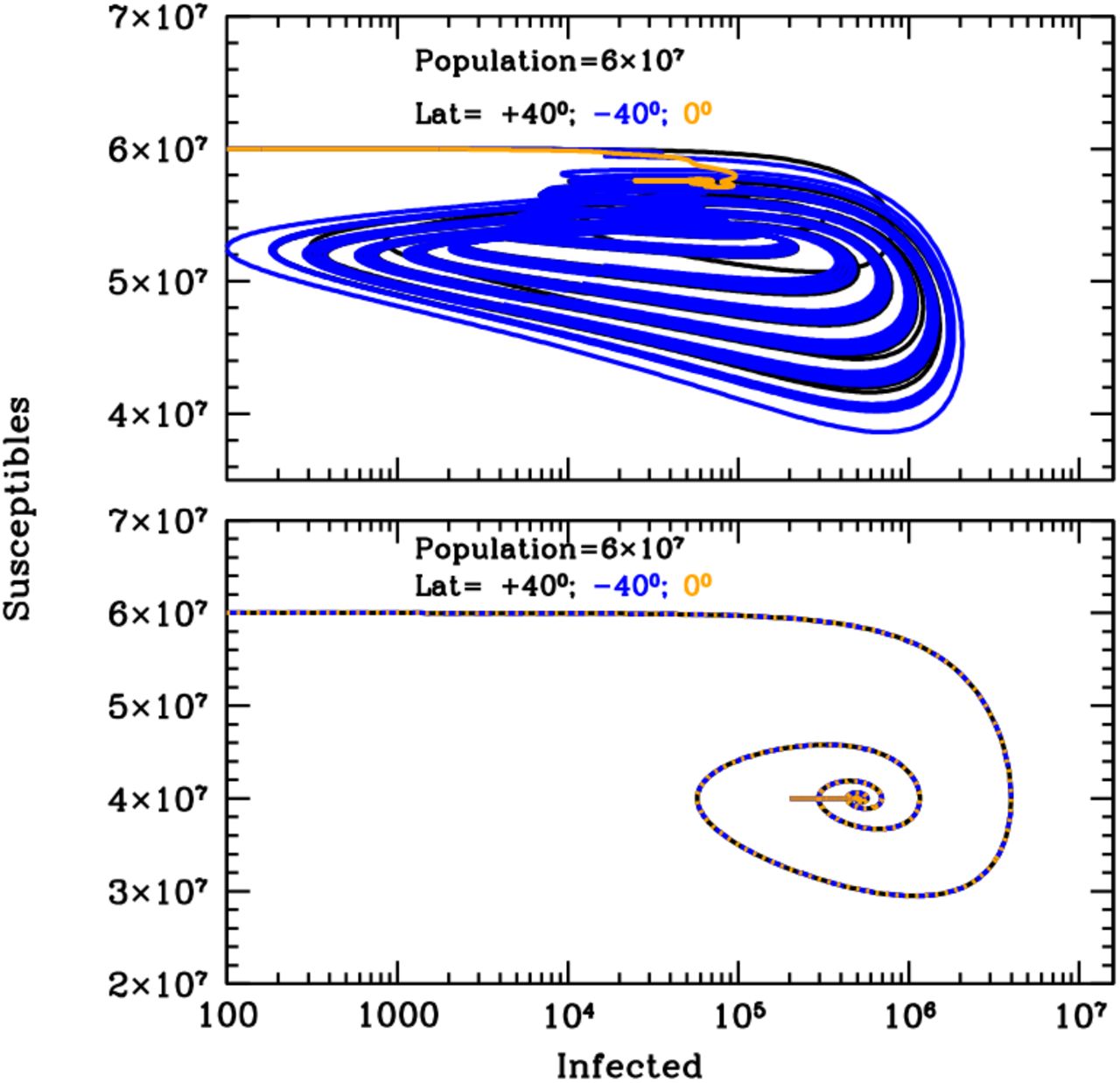
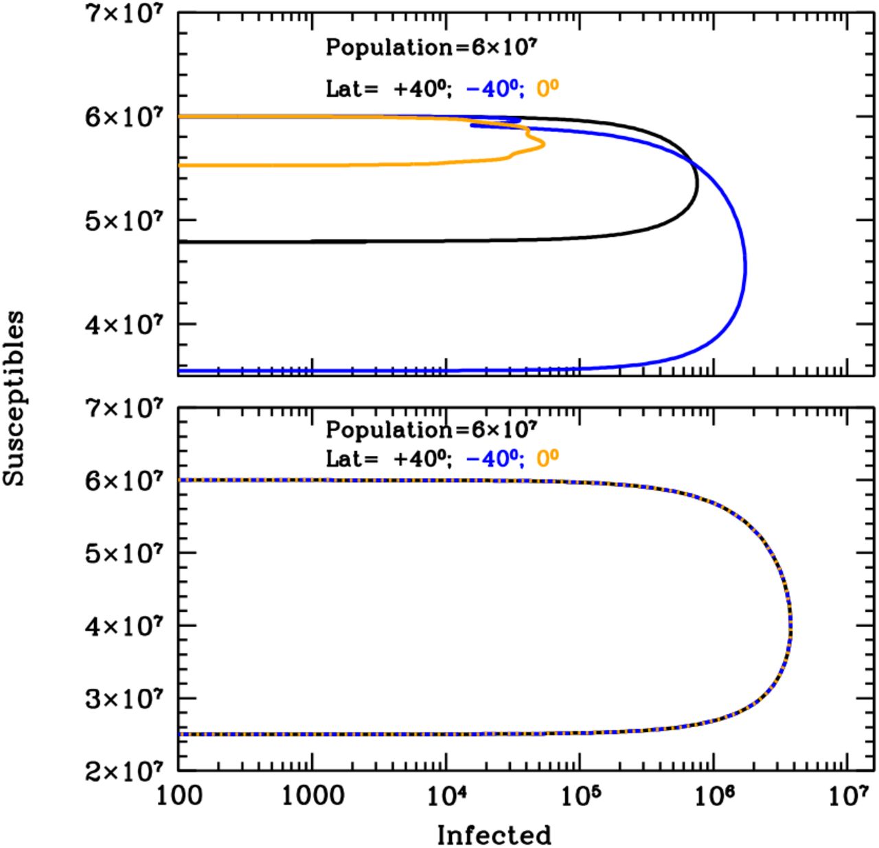
Figure 1 shows the curves of growth of the infected individuals in the three latitude groups over the first 20 years of an influenza epidemics with (top panel) and without (bottom panel) solar-pump (see caption for details). When the solar-pump is not active (bottom panel) the growth (and decline) of epidemics proceeds identically at all latitudes (black, blue and orange curves are superimposed to each others). The period of oscillations, in this case, resonates solely with the inverse of the LOI rate (the time it takes for previously infected individuals to become again susceptible), the strength of epidemics declines from cycle to cycle, and the disease dies out completely in less than 10 years. When the solar-pump is active, instead, the reproductive number undergoes small infra-day variations (whose exact magnitude depends on the particular time of the year and Earth’s latitude) that do not significantly change its daily average value, but progressively drive the modulation of epidemic oscillations to match the seasonal solar period (Fig. 1, top panel). The north (black), south (blue) and tropical (orange) groups differentiate immediately, and after a few cycles (lasting a total of about 5 years) are perfectly regulated on biannual periodicity, with phase shifted in time by 6 months in the north versus south hemisphere and the tropical group undergoing fast and continuous moderate bursts of epidemics roughly every six months. The biannual oscillations at latitudes ±40 degrees, last for a few tens of years, and then synchronize with the yearly solar-irradiation seasonal period (see figure’s caption for details). The cycles can run unperturbed for centuries, as shown in the top panel of the Susceptible versus Infected (SI) phase-diagram of Fig. 2, where the first 100 years of endemic diseases are drawn (see Figure’s caption for details).

Susceptible versus actual infected phase diagrams of the influenza outbreak run described in Fig. 1’s caption, with (top panel) and without (bottom panel) active solar-pump. The first 100 years of the epidemics are plotted (every other 10 years, in the top panel, for easier visualization). When the solar-pump is not active (bottom panel), the curves are the same at all latitudes and the cycles of epidemics die out quickly (essentially in 3-4 cycles) because of lack of supply among the susceptible population. When the solar-pump is switched on (top panel) the resonant mechanism builds up seasonality quickly. During the first 50 years, and at latitudes of ±40 degrees (black and blue curves), the susceptible population at each time oscillates between 65–98% of the population, and the instant fraction of infected people over susceptible, at the peaks, reach maximum values of about 4.5%. At the equator oscillations are much milder (orange curve): after a first long-duration cycle, the susceptible population at each time settles at a fraction of about 98% of the total while infected people oscillates steadily between 0.06–0.2% of the susceptible population.
Our second case-study B aims to model the recent SARS-CoV-2 pandemics outbreak under the different assumptions tested in this work, and allows us to gain insights on possible future scenarios. As for case A, we use the three groups at latitudes 40°-north, 40°-south and the equator, and run simulations both with and without the solar forcing term and for a LOI rate of γin=0.0055 (but see also the Supplemental Material [12] for a comparison with the cases with LOI rates γin=0 and γin=0.00055). However, for case B we also compare our north-hemisphere simulation with the SARS-CoV-2 data for Italy (central latitude +41.5 degrees) observed from 24 February 2020 through 4 July 2020 (see the Supplemental Material [12]). To do so, we introduce, for all groups, two additional external forcing terms that modulate the contact rate β (chosen to be 0.3, to reproduce the observed – in virtually every monitored country – initial exponential growth rate): a ‘lockdown’ term and a ‘phase-2’ term (see Fig. 3’s caption and the Supplemental Material [12]).

Simulation of the curves of growths of the daily new infected for the first 3 years of the SARS-CoV-2 pandemics at three different latitudes on Earth, +40 degrees north (black), −40 degrees south (blue) and the Equator (orange), with (top panel) and without (bottom panel) active solar-pump. Model parameters are t0=January 5th 2020, tend=t0+100 years, R0=3.0, γout=0.1, γin=0.0055, µ=0.01 and external lockdown and phase-2 starting on 11 March 2020 and 10 May 2020, with halving and doubling times of 46 and 180 days, respectively. Black points are SARS-CoV-2 data for Italy from 24 February 2020 through 4 July 2020, smoothed over a 7-day moving average. For the active solar-pump case (top panel) all curves of growth of new daily infected have been scaled down by a factor of 10 to let the +40° curve (black) match the Italian data of the current outbreak: the model closely matches observations. In the non-active solar-pump case (bottom panel) model curves needs to be scaled-down by an unrealistically high factor of 300, and only the climbing phase of the outbreak in Italy can be reproduced. Yearly oscillating dotted curves at the bottom of the top panel are UV-B/A lethal-exposure estimated for Covid-19.
With the particular initial setting described in the caption of Fig. 3, the simulation with active solar-pump and fast antigenic-drift (γin=0.0055) reproduces extremely well the curve of growth of the observed daily number of infected in Italy (Fig. 3, top panel, black infected curve and data), with an under-sampling factor of 10 (i.e. observed infected are one tenth of actual infected). Preliminary results from serological tests on a statistically selected sample, confirm this average under-sampling factor in Italy1.
The bottom panel of Fig. 3 shows the same simulation when the solar-pump is not active (curves of growth from the three latitude groups are superimposed to each other). However, here the under-sampling factor needed to fit the initial exponential phase of the growth of contagions in Italy is an unrealistic factor of 300. Moreover, the declining phase of contagions, with no solar-pump is too fast to reproduce the Italian data. The much smaller absolute number of daily infected in the simulation shown in the top-panel of Fig. 3, compared with that of the bottom panel (under-sampling factor of 10, versus 300), and the slower decay of daily detected infections, are due solely to the daily effect of the solar-pump. The fast-decay in the inactive solar-pump case is a direct consequence of the much larger ‘consumption’ of susceptible individuals during the growth of contagions (compare top and bottom panels of Fig. 4).

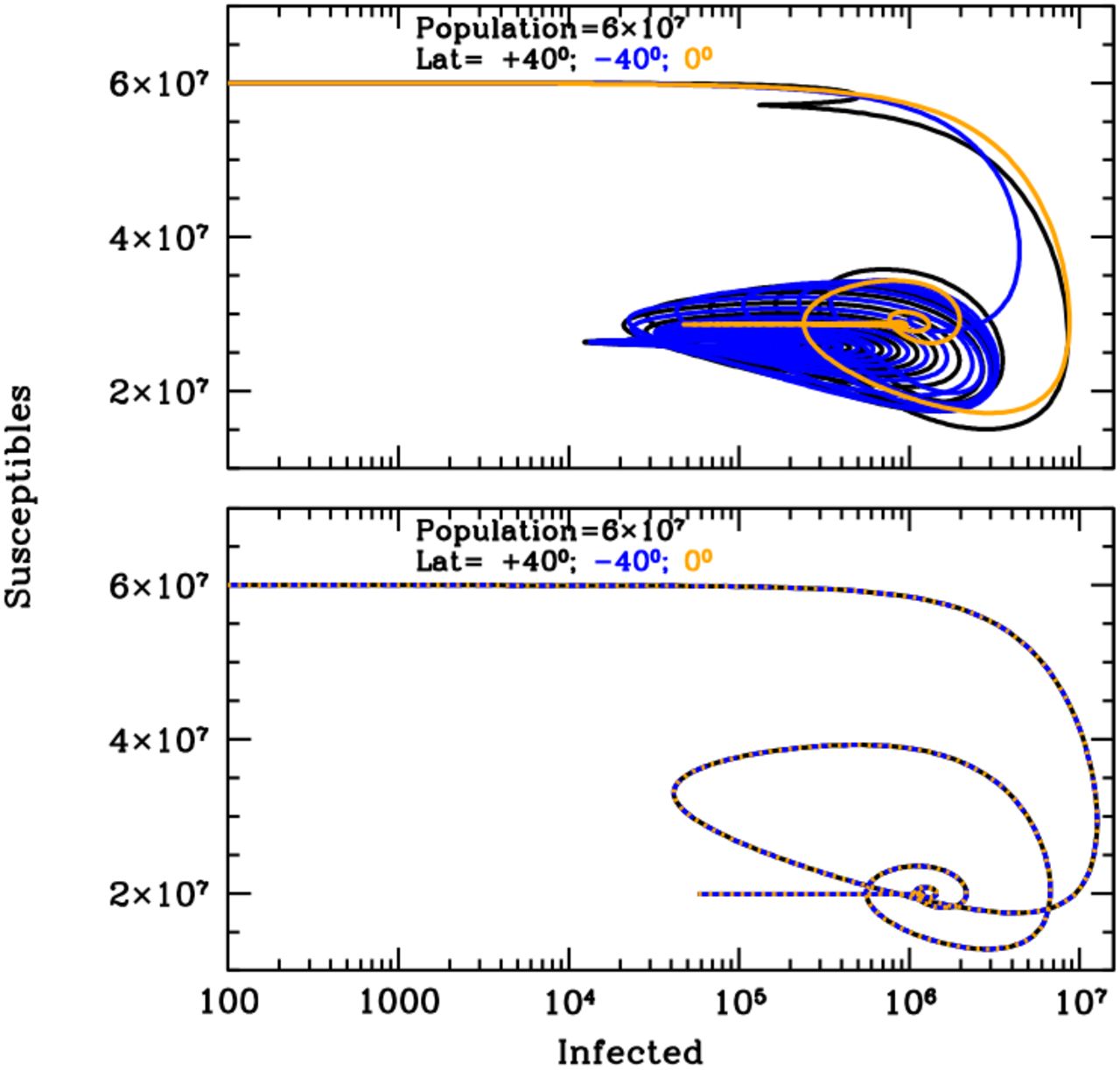
Susceptible versus actual infected phase diagrams of the SARS-CoV-2 pandemic outbreak run described in Fig. 3’s caption, with (top panel) and without (bottom panel) active solar-pump. The first 10 years of the possible evolution of the epidemics are plotted. When the solar-pump is not active (bottom panel), the curves are the same at all latitudes and the cycles of epidemics die out in 4 cycles because of lack of supply among the susceptible population. Considering the effect of solar-pump (top panel) makes the epidemics evolve quickly to endemic at all latitude. After the first 3 cycles, and at latitudes of ±40 degrees (black and blue curves), the susceptible population at each time oscillates between 33–55% of the population, and the instant fraction of infected people over susceptible, at the peaks, reach maximum values of about 12%. At the equator the amplitude of oscillations is much smaller (orange curve), the susceptible population at each time settles at a fraction of about 50% of the total while infected people oscillates steadily between 0.2–3.5% of the susceptible population.
The sun has also the effect of reducing by almost one and two orders of magnitude, respectively, the number of infected individuals observed from February through May, in the South and tropical group, with respect to the North group, which is exactly what has generally been observed during the SARS-CoV-2 pandemic (Fig. 3 top panel). The curve of growth of the South group, however, starts climbing again in May and, if no additional distancing measures are adopted, should have a second and much higher peak in October, towards the end of the South winter (Fig. 3, top panel). In the north hemisphere, instead, this simulation (but see the Supplemental Material [12] for an alternative scenario) predicts that the epidemics should see a minimum in July-August and start again aggressively in October-November, while tropical countries will see a second prolonged and much stronger outbreak from July 2020 through January 2021. Subsequently, under these conditions, the epidemics will start adjusting to the solar cycle and less aggressive outbreaks (daily number of actual infected between ten thousand and hundred thousand) will repeat cyclically for tens of years (Fig. 4).
While only an external seasonal driver (like the solar-pump) can explain the qualitative differences observed when the strength of the SARS-CoV-2 pandemics is compared in countries located in the north, tropical and south hemisphere (compare, e.g. top and bottom of Fig. 3), the particular set of model parameters we used to match the Italian data of the ongoing SARS-CoV-2 epidemics (see Fig. 3’s caption for details), is obviously not unique. In particular, these depend on the starting time of the epidemics and the actual efficiency of the Solar effect, which, in turn, depends on the exact knowledge of the virus’ UV-C lethal dose D0 (see the Supplemental Material [12]), the way this is delivered and the time the virus (in aerosol or surfaces) remains exposed to the dose. Accurate modeling of this phenomenon is beyond the scope of this work. However, in the Supplemental Material [12] we show the comparison with a drastically different solar-pump efficiency (3 times lower than in the case of Fig. 3 and 4) to highlight the potential predictive power of the model for the SARS-CoV-2 epidemics, which offers the opportunity not only to clearly distinguish between low- and high-efficiency solar-pump scenarios, but also to evaluate the magnitude of the effect.
Our model is able to reproduce in a particularly precise way the seasonality of influenza-like epidemics and its phase-latitude dependence, and can explain the qualitative differences generally observed when the strength of the SARS-CoV-2 pandemics is compared in countries located in the north, tropical and south hemisphere. Moreover, comparison with SARS-CoV-2 data at different latitudes over the next few months, should tell us about the importance of the solar-pump effect in modulating the spreading of this disease, although the exact quantification of this effect will require dedicated laboratory measurements of the inactivation of the virus when exposed to solar-like spectra as well as other important parameters like average life-time of the virus in aerosol or surfaces, its transport in wind or low-atmosphere currents, etc. This is beyond the scope of this work, whose aim is to show the potential of solar radiation in modulating the short- and long-term evolution of epidemics outbreaks and demonstrate that the, unavoidable, infra-day (minute timescales) resonant mechanism naturally offered by the solar-pump, can efficiently synchronize with internal LOI rates to explain the course of epidemics on much longer timescales.
The work presented in this paper has been carried out in the context of the activities promoted by the Italian Government and in particular, by the Ministries of Health and of University and Research, against the COVID19 pandemic. Authors are grateful to INAF’s President, Prof. N. D’Amico, for the support and for a critical reading of the manuscript. Authors are also grateful to Dr. M. Elvis for critically reading the papers and providing useful comments and suggestions. A research grant from Falk Renewables partially supported this work.
Data Availability
All data used in the manuscript are publicly available, at https://github.com/CSSEGISandData/COVID-19 (SARS-CoV-2 data) and http://www.temis.nl (solar irradiation data)
Supplemental Material
Our Deterministic Model
We adopt a simple deterministic SIRS model, in which the Susceptible population (S) interacts not linearly with Infected (I) at a rate β, Recovers (R) or dies (D) with rates γout and µ, respectively, and can become again susceptible (loses immunity) with a rate γin:
 We wrote a simple Fortran-90 routine that solves this system of differential equations (non-linear only in I and S) iteratively, for arbitrary values of the model parameters. We adopt a time-unit of 1 day and, at each iteration, perform infra-day integrations.
We further introduce three optional external forcing terms that act on the reproductive number Rt by attenuating or amplifying it on timescales of 1 day (lockdown and phase-2 terms) and minutes (solar-pump) and may be switched on and off during runs.
Lockdown and Phase-2 terms are modeled with exponential functions with, respectively, halving and doubling times that are free parameters of the model. The lockdown attenuation ends when phase-2 starts, and phase-2 amplification ends when Rt reaches the original value R0 characteristic of the disease.
The solar-pump forcing term is modeled by following the sun radiation curves as a function of Earth’s latitude, day of the year, and time of the day. Solar curves (Fig. 1) are functions of the solar height angle α (complement to the Zenith angle: i.e. α=90 degrees at local noon) that, in turn, depends on Earth’s latitude φ, sun’s declination δ, day of the year d and the time of the day h. Solar curves modulate daily with sin(α) and have maximum amplitudes and widths that depend on φ, d and h, as shown in Fig. 1, where the Rt attenuation factor (1 – sin(α)) is plotted (for α>0, i.e. during daytime) versus h for the 15th day of first 6 months of the year. In each panel of Fig. 1, different curves correspond to different Earth’s latitudes (in steps of 5 degrees), from 25 to 90 degrees north (black), −25 to −90 degree south (blue) and −25 to +25 degrees (orange).
Efficiency of the solar-pump
For the solar virus-inactivation mechanism to be effective in modulating the disease’s transmission and settling the duration and recurrence of epidemics, both direct contact (e.g. through exposed surfaces) and airborne transmission have to play a role (as is the case for most respiratory diseases, e.g. [1] and references therein) and the time needed for aerosol particles to gravitationally settle has to be comparable or longer than the typical UV-B/A virus’s lethal time [2]. This is probably not true (in still air) for the largest (∼100 µm in size) and thus heaviest droplets produced in coughs and sneezes, where the gravitational settling time is of the order of few seconds [3], but can certainly be the case for significantly smaller, micron or sub-micron size, aerosol particles (like those that commonly contain the influenza virus, e.g. [4]) that can survive in still air for longer than 12.4 hours [4].
The efficiency of the solar-pump effect depends also on internal virus properties, namely on the lethal time τ0 needed to deliver the UV lethal dose D0 (defined as the UV-C fluence needed to inactivate 63% of the virus) for the given virus [2]. At local noon (the peak of the daily solar curves of Fig. 1) typical UV-B/A solar intensities on Earth range from 0.9–18 J m-2 min-1 in the north and south hemispheres between winters and summers, respectively, and are roughly constant at the equator throughout the year with a mean value of ∼ 18 J m-2 min-1. Folding these intensities through the action spectrum (i.e. the ratio of the virucidal dose of UV radiation at a given wavelength to the lethal dose at 254 nm) of [5], yields to lethal UV-B/A intensities of ∼0.05–1 J m-2 min-1. For Covid-19 we measured a three orders of magnitude inactivation dose of 37 J m-2 [24], which translates into D0=4.8 J m-2. This value is used to produce the lethal-time dotted curves of Figures 1 and 3 of the manuscript and Fig. 3,5,7 and 9 of this Supplemental Material, which oscillate between 5-100 minutes at local noon depending on latitude and the time of the year.
Solar-Pump Efficiency Dependence
To check the dependence of the evolution of the SARS-CoV-2 epidemics on the solar-pump efficiency, we simulate a three times lower solar-pump efficiency by squeezing the amplitude of the solar-pump curves of Fig. 1 by a factor of 3. Figure 2 shows the results of such simulations for the three groups at ±40 degree latitudes and the Equator and for a set of model parameters that, as for the case of Fig. 3 in the manuscript, matches reasonably well the Italian SARS-Cov-2 curve of growth of contagions (see figure’s caption for details) from the start of epidemics through 4 July 2020 and with an under-sampling factor of 25 (probably too high, based on preliminary results from serological tests in Italy). Even with such reduced efficiency the solar-pump is able to produce significant differences in the curves of growth of the epidemics at ±40 degree latitudes and at the Equator (black, blue and orange solid curves in Fig. 2), which, however, start to synchronize with seasons only after a few cycles. Moreover, short-term predictions, at all latitudes, differ significantly from the case with higher solar-pump efficiency (Fig. 3 in the manuscript). Italy (and in general, countries located at ∼ ±40 degrees), where distancing measures have now greatly being relaxed, should start seeing a strong increase in the number of new daily infected in September, and this should continue, in absence of distancing measures, through the end of January 2021, to then drop quickly in spring 2021 and restart again a few months later, in summer 2021. In the case discussed in the manuscript, instead, the epidemic in Italy should have a second sharp peak in October 2020 and then die out quickly just before the beginning of winter 2020. Such different predictions depend mainly (in absence of further distancing measures), on the relative significance of the solar mechanism, and thus offer the opportunity not only to clearly distinguish between the two scenarios, but also to evaluate the magnitude of the effect.
LOI Rate Dependence
In Fig. 1–4 of the manuscript we show curves of growth and phase diagrams of epidemics for a relatively fast LOI rate, compared with the seasonal frequency. Here we show two comparison cases, for a LOI period much longer than seasonal (γin=0.00055, i.e. 5-year period) and for γin=0 (no antigenic-drift).
Influenza
When γin=0.00055 (Fig. 3 and 4) oscillations are erratic and chaotic during the long settling period: destructive resonance between the LOI rate and the Solar cycles acts differently in the three latitude groups, and if no group mixing is introduced the intense bursts of epidemics are initially separated by the inverse of LOI rate. This separation progressively shrinks at all latitudes as the continuous solar-pumping imposes its rhythm, and becomes strictly seasonal at all latitudes in about 40-50 years. The squeezing of the time intervals between outbreaks, is visible also when the solar-pump is not active (Fig. 3, bottom panel). This is because, as new outbreaks develop, the reservoir of susceptible made available by previous LOI cycles and the number of people still infected at any time are sufficient to trigger new bursts at earlier times. However, in this case, the strength of each outbreak decreases smoothly and systematically with years, and in about 70 years the reservoir of susceptible at each time completely empties and the epidemics die out. Moreover, again, the three latitude groups behave identically, which is not observed.
When γin=0 (no antigenic-drift: Fig. 5 and 6), the solar-pump cannot, alone, sustain stationary epidemic cycles, but strongly modulates the course of epidemics during the first three years in the north and south hemisphere and over a long period of about 8 years in the tropical area (Fig. 5, top panel). By contrast, when the solar-pump is not active the epidemics develop identically at all latitudes and last for a single 1-year cycle (Fig. 5 and 6, bottom panels).
SARS-CoV-2
Should recovered people preserve their immunity against Covid-19 (γin=0 case), UV photons from the Sun may still be able to amplify contagions during autumns/winters and produce one or two additional waves of the SARS-CoV-2 epidemics at all latitudes (Fig. 7 and 8). However, after three years (and only 2-3 cycles), in absence of antigenic-drift or cross-mixing between groups at different latitudes, the epidemics will die out. Finally, as for case A (influenza), at the much slower LOI rate γin=0.00055 (LOI period of 5 years), the seasonal cycle takes much longer to stabilize, and oscillations proceed at intermittent intensities both in the north and south hemisphere (with different phases) for tens of years, and then finally synchronize to the Solar cycles on timescales longer than 50 years (Fig. 9 and 10).
Solar UV Data
In our study, to compute lethal times τ0, we use Solar UV data made available by the Tropospheric Emission Monitoring Internet Service (TEMIS) archive1. TEMIS is part of the Data User Programme of the European Space Agency (ESA), a web-based service that stores, since 2002, calibrated atmospheric data from Earth-observation satellite. TEMIS data products include measurements of ozone and other constituents (e.g. NO2, CH4, CO2, etc.), cloud coverage, and estimates of the UV solar flux at the Earth’s surface. The latter are obtained with state-of-the-art models exploiting the above satellite data.
SARS-CoV-2 Pandemics Data
We collect SARS-CoV-2 data pandemics for Italy from the on-line GitHub repository provided by the Coronavirus Resource Center of the John Hopkins University (CRC-JHU)2. Such data are provided daily by the Italian civil-defense department. CRC-JHU global data are updated daily and cover, currently, the course of epidemics in 261 different world countries, by providing the daily cumulated numbers of Confirmed SARS-CoV-2 cases, Deaths and Healings. We use CRC-JHU data run from 24 February 2020 (recorded start of the epidemics in Italy) through 4 July 2020.
Black points of Fig. 3 of the manuscript and Fig. 2, 7 and 9 of this Supplemental Material, are the 7-day moving average of the daily number of confirmed SARS-CoV-2 cases in Italy.

Attenuation functions for the reproductive number Rt, due to the daily solar action. Each panel show solar attenuation curves for 36 Earth’s latitudes between −90 and −25 degrees south (blue), −25 – +25 degrees (orange) and 25–90 degrees north (black) at the 15th day of each of the first 6 months of the year, as labeled. The plotted function is (1 – sin(α)), where α is the solar height angle (complement to the Zenith angle: i.e. α=90 degrees at local noon) that depends on Earth’s latitude φ, sun’s declination δ, day of the year d and time of the day h.

Same as Fig. 3 in the manuscript, but for a solar-pump with efficiency 3 times lower (parameterized here by three times longer lethal times: dotted curves) and model parameters: t0=January 15th 2020, tend=t0+100 years, R0=3.0, γout=0.1, γin=0.0055, µ=0.01 and external lockdown and phase-2 starting on 11 March 2020 and 20 April 2020 (20 days earlier than the actual official Phase-2 date in Italy), with halving and doubling times of 25 and 370 days, respectively. All curves of growth of new daily infected have been scaled down by a factor of 25 to let the +40° curve (black) match the Italian data of the current outbreak: the model closely matches observation, however, short-term predictions dramatically differ from the case plotted in Fig. 3 of the manuscript (see text for details).

Same as Fig. 1 in the manuscript, but for a slow LOI rate of γin=0.00055. As for the fast LOI rate case, when the solar-pump is active (top panel) constructive resonance eventually (after ∼40 years) builds-in regular sun-modulated oscillations already after the first 2 cycles, and the strength of the seasonal outbreaks adjust to constant values that depend on latitude. However, during the first 30-40 years, intensive outbreaks are sporadic at all latitudes and typically repeat for 2-3 consecutive years. Without solar-pump (bottom panel) the cycles are the same at all latitudes and are fed by LOIs only till the available number of susceptible is sufficient. The strength of the outbreaks decreases steadily with time, and time-intervals between peaks squeezes, from the inverse of the LOI rate to ∼0.2 times that.

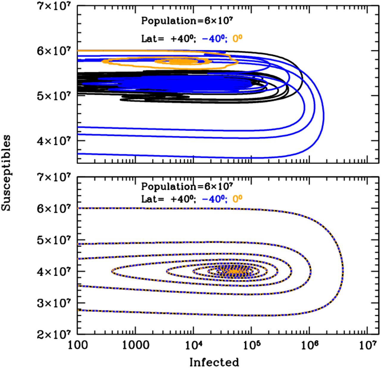
Same as Fig. 2 in the manuscript, for the model of Fig. 3 and for the entire duration of the simulation (100 years). The LOI mechanism alone is able to support a few cycles of the epidemics (bottom panel), but these decreases systematically in strength and eventually die out. Switching the solar-pump on (top panel) allows the system to remain active for the entire duration of the simulation and to stabilize after 30-40 years to susceptibility fractions of ∼85% and 97%, at all times, at ±40 degrees and at the Equator, respectively. Correspondingly, the fraction of actual infected over the susceptible population, oscillates steadily between 10−5 – 0.002 and 5×10⁻⁵ – 1.7×10⁻⁴, at ±40 degrees and at the Equator, respectively.

Same as Figure 3 for the first 8 years of an influenza-like epidemics with zero LOI rate. When internal dynamics is absent (no LOI) the epidemics cannot become endemic. However, when the solar-pump is active (top panel) UV photons from the sun are able to modulate the outbreak and prolong it for a few cycles (top panel). A couple of bursts are seen at ±40 degrees, whereas a single long, mild and Sun-modulated epidemics develop at the Equator and last for about 6 years. Without solar-pump (bottom panel) a single intense episode is seen at all latitudes.

Same as Fig. 4, for the model of Fig. 5 and for the entire duration of the simulation (100 years). The epidemics are not sustained by LOI and die out quickly. However, the total number of people infected before the outbreaks are over, depends on whether the solar-pump is active (top panel) or not (bottom panel). With epidemics starting during north-hemisphere winters (as in our models), latitude +40 degrees reaches a maximum infected over susceptible fraction of 1%, while this fraction is four times larger at −40 degrees and about ten times smaller at the Equator.

Same as Figure 3 in the manuscript, but for a zero LOI rate (γin=0). With these parameters, the model is not able to adequately match the Italian data of the outbreak (black points), even when the solar-pump is active (top panel). However, only when UV photons are considered (top panel), can the model reproduce the observed differences in geographical spread of the pandemics. Should recovered people preserve their immunity against Covid-19, UV photons from the Sun may still be able to amplify contagions during autumns/winters and produce one or two additional waves of the SARS-CoV-2 epidemics at all latitudes. This cannot happen in absence of UV photons (bottom panel), even after lockdown measures are loosened.

Same as Fig. 4 in the manuscript, for the model of Fig. 7 and for the entire duration of the simulation (100 years). Both in the active (top panel) and non-active (bottom panel) solar-pump cases, the epidemics are not sustained by LOI and die out quickly. However, when UV photons are considered, the epidemics last longer (a total of three years at all latitudes). With epidemics starting during north-hemisphere winters (as in our models), and in absence of additional lockdown measures, three full cycles develop +40 degrees, two at −40 degrees, and a single, asymmetric cycle at the Equator.

Same as Fig. 7, but for the slow-rate LOI scenario (γin=0.00055, or 5-year period) and for the first 50 years of the simulation. Both with (top panel) and without (bottom panel) the solar-pump, cycles proceed driven by the slow-rate reappearing vulnerability of the immune system, with decreasing periods at all latitudes. When UV photons are considered the initial epidemics’ bursts are generally intense and erratic, especially at north and south altitudes, and become steadily recurring and stabilize to the seasonal cycle after 25-50 years depending on latitude (and in absence of cross-mixing population), fortunately with moderate strength.

Same as Fig. 8, but for the model of Fig. 9. Should LOI happen on a long timescale (5 years in this simulation), the presence of UV photons from the sun (top panel) would make the first 8-10 epidemics bursts in the north hemisphere, particularly intense. The fraction of actual people infected at any time over the susceptible population, would reach peak values of 10% during the first 25 years, and would then stabilize, oscillating within the range 0.03–2.4% (at latitudes ±40) and 0.2–1% (at the Equator), for the next 75 years.


