A random forest model for forecasting regional COVID-19 cases utilizing reproduction number estimates and demographic data

2.1 Data Acquisition

Our time-series datasets begin on 03/31/2020 for 3068 U.S. CCEs with complete, consistent data that could be processed without error in our downstream pipelines. To normalize testing and case counts by population, these metrics were converted to incidence rate (IR) using the 2018 U.S. Census CCE-level population estimates in Eq. 1.

2.2 Generation of R_t and Case Alignment Forecast Features

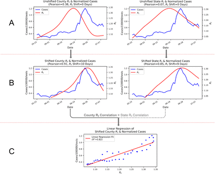
For any given date in every U.S. CCE, we forecasted R_t and testing-normalized cases for 1, 2, 3, and 4 weeks into the future. First, a testing-normalized COVID-19 cases time-series was generated by dividing the “Weekly case increase” feature by the “Daily tests increase” feature (see Table 1). The normalized cases time-series and the “Daily estimated R_t” feature were used to generate R_t and case-prediction features, as shown in Fig. 1. All linear regression models were implemented with the linear_model.LinearRegression module [28].

• Download figure
• Open in new tab

Figure 1: R_t and case prediction feature generation for a CCE.

This procedure is repeated for 7-, 14-, 21-and 28-day forecasts. In Fig. 1A and Fig. 1B, R_t for the CCE and its state are both separately considered; whichever achieves the highest Pearson correlation of any forward shift x that is <50 days (i.e. optimal shift) is used for the regression model in Fig. 1B. The extrapolation in Fig. 1E is calculated by linear regression models trained on the last 14 defined values of each curve; curves are extrapolated to the target end date (i.e. 7, 14, 21, or 28 days in the future). For Fig. 1F, curves in prediction time have forecasted values relative to real time; thus, for 28-day forecasts, values are those forecasted 28 days into the future.

2.3 RF Training and Forecasting

The dataset used to train and validate the RF forecasting models includes all features in Table 1 for each U.S. CCE; however, “Weekly case increase” and “Daily estimated R_t” features were replaced with the Fig. 1F features for 7-, 14-, 21-, and 28-day forecasts. Thus, the preliminary forecasts were used as features to generate the final forecasts. All features were normalized by removing their mean and scaling to unit variance. For each Sunday from 11/01/2020 to 01/10/2021, we trained and validated RF forecasting models via incremental learning. Thus, we filtered out feature data that occurs on or after the Sunday of interest, but later Sundays will have more feature data than earlier Sundays. Then, we randomly split the feature data for a given Sunday into a training subset and a validation subset with a 9:1 ratio, respectively. The training subset is used to train a RF regression model for each forecast timepoint (7, 14, 21, or 28 days into the future); the target outcome was the “Weekly case increase” from Table 1 shifted backwards to represent future cases on the forecast timepoint. The validation subset is used to ensure that trained RF models do not overfit the training subset. Finally, data for the Sunday of interest is input to the trained RF models to generate forecasts for each forecast timepoint.

RF regression models are ensemble machine learning algorithms that were first described by Breiman [12]. They create multiple regression trees trained on unique bootstrap samples of the training dataset with a random subset of the input features. The output of all trees is averaged to create the final projection. We used the Scikit-learn (version 0.23.2) implementation with default hyperparameters and 20 estimators [28].

2.4 Model Evaluation

The permutation importance of all features input into the RF models was calculated as described by Breiman as the decrease in mean squared error of the model when a feature of interest is randomly shuffled [12]. We used two metrics, MAE and R-squared (R²), to evaluate the accuracy of our model’s forecasts relative to actual case counts for both the training dataset and forecasts outside of the training dataset. These metrics are calculated as follows: We also used these metrics to calculate the error for equivalent forecasts by the JHU Infectious Disease Dynamics group (IDD), the JHU Applied Physics Lab (APL), and One Quiet Night (OQN) forecasting models [29, 30, 31]. These were selected as they are parts of the U.S. Centers for Disease Control and Prevention (U.S. CDC) ensemble model, have relatively high performance, and forecast for a large breadth (2349) of U.S. counties along with the RF model [32].

3.1 Analysis of R_t and Case Alignment Forecasts

When the case time-series for a CCE was normalized by population and state-level testing data, it often showed a very similar shape to the CCE and/or state R_t time-series, as shown in Fig. 1. This should be expected, as both time-series indicate new infection load over the course of an epidemic, although R_t lags behind cases, which we suspect is because R_t represents infection load in the present moment, but these infections will not be detected via testing until much later due to viral incubation periods of 2-14 days and test result reporting delays [33]. In the 01/10/2021 dataset, the average optimal shift for the most highly correlated R_t time-series, whether state or CCE, was 34 days forward.

However, there were many CCEs where this relationship was weak. We observed that 1782 CCEs’ selected, optimally shifted R_t time-series have a Pearson correlation with the case time-series < 0.5. They also have a mean population density of 89 people/mi², vs. the 273 people/mi² mean over the entire set of 3068 CCEs. Thus, we attribute the low correlations to poor and/or inconsistent testing efforts and data quality in rural CCEs. Further supporting this is our observation that in CCEs where we select their state’s R_t time-series as opposed to their own, the mean population density is also relatively low at 210 people/mi².

In concurrence with Omori et al., we found that normalization of the case time-series with testing data is critical to expose underlying changes in COVID-19 progression, as seen in Fig. 2 [34]. However, our approach is limited by use of state-level testing data as opposed to CCE-level testing data, which was inaccessible to us. However, state-level testing data has the advantage of including individuals who are not tested in their CCE of residence due to inequity in regional testing access.

• Download figure
• Open in new tab

Figure 2: R_t Time-Series’ Lag Behind Case Time-Series Used to Forecast Cases in Lag Period.

In Harris County, TX, when the CCE R_t time-series from 05/22/2020 to 07/10/2020 has a maximum Pearson correlation with the CCE’s testing and population normalized case time-series for the same period when shifted forward 10 days (B); also, this correlation is higher than that obtained by any shift of the state R_t time-series. Thus, the shifted CCE R_t time-series is linearly regressed against cases (C). This model is applied to unshifted CCE R_t time-series to generate a case-prediction time-series; the last 10 days of both these time-series are predictive of the next 10 days of cases beyond 07/10/2020.

3.2 RF Feature Prioritization and Training Performance

On average over the 11 epi weeks, RFs always prioritized population-normalized, state-level test numbers, test positivity, and case and R_t alignment forecasts as seen in Fig.3. This validates the model, as these features most directly measure COVID-19 progression. Importantly, of all 8 alignment forecasts, those for the desired forecast target were always prioritized highest. Conversely, demographic, population health, and population mobility features are relatively inconsequential; on average across Fig. 3A-D, these 46 features’ share of the total sum of all 56 features’ permutation scores is just 14.33%.

• Download figure
• Open in new tab

Figure 3: Top 7 RF Features for Each Forecast Target.

For each forecast target, RF feature permutation importances were averaged over all 11 epi weeks and the top 7 features are shown in the subfigures above along with their standard deviation as error bars.

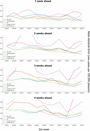
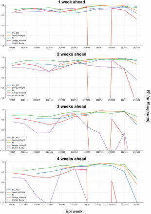
On the training datasets for all 4 forecast targets and all 11 epi weeks, R² was very stable, averaging 0.97 with a standard deviation of 0.00. For the corresponding validation datasets, R² fell to 0.92 with a standard deviation of 0.02. Thus, overfitting is not extreme and, considering the RFs’ relatively high MAE and R² on actual case data in comparison to other models as seen in Fig. 4-5, is not detrimental to our objectives.

• Download figure
• Open in new tab

Figure 4: Performance Evaluation Using MAE.

The errors between projections and real number of incident cases were calculated using Eq. 3. The y-axes of the graphs have been limited so that all models can be visually compared.

• Download figure
• Open in new tab

Figure 5: Performance Evaluation Using R².

As with Fig. 4, the y-axes of the graphs have been limited. The proportions of variance between projections and observed values were evaluated using Eq. 2. We notice that there are large anomalies in the weekly R² of the Google_Harvard and JHUAPL_Bucky models after epi week 202051; however, for the sake of complete comparison, all weeks for all models are shown.

3.3 RF Forecasting Performance vs. Other Models

As may be observed in Fig. 4 and Fig.5, over the 11 reference weeks for which forecasts were generated by the RF models, MAE and R² remain relatively consistent compared to the OQN and JHU models. The RF’s R² is competitive with and often higher than the R² for other models, notably November 2020. Cases in November were harder to model accurately, as November saw a 40% increase in cases in the 3068 counties in its fourth week relative to its first week, whereas December only saw an 8% decrease in cases for its equivalent comparison period. Periods of relatively low performance are generally shared by all models, indicating that case load changes during these weeks are simply less predictable.

For each epi week, case projections from each model were collected and compared to actual cases that occurred during these weeks as reported by JHU [18]. The results were calculated and visualized in Fig. 4-5.

The JHU IDD and APL models are SEIR models [29, 30], whereas the OQN model applies a linear regression model to each CCE [31]. The distribution of output from a model exclusive to a CCE will be skewed towards the distribution of its training dataset labels, which may be a factor explaining OQN’s low MAE. On the other hand, the RF model forecasts for all counties, affording it a larger dataset which possibly contributes to its relatively high, stable fit to the actual cases as indicated by its R².