
Abstract
Drug resistance is a problem in many pathogens, including viruses, bacteria, fungi and parasites (Murray et al. 2022). While overall, levels of resistance have risen in recent decades, there are many examples where after an initial rise, levels of resistance have stabilized (Krieger et al. 2020; Colijn et al. 2009; Diekema et al. 2019; Rhee et al. 2019; Rocheleau et al. 2018). The stable coexistence of resistance and susceptibility has proven hard to explain (Krieger et al. 2020; Colijn et al. 2009; Cobey et al. 2017; Kouyos, Klein, and Grenfell 2013; Blanquart et al. 2018). Here, we show that a simple stochastic model, mathematically akin to mutation-selection balance theory, can explain several key observations about drug resistance: (1) the stable coexistence of resistant and susceptible strains (2) at levels that depend on population-level drug usage and (3) with resistance often due to many different strains (resistance is present on many different genetic backgrounds). The model works for resistance due to both mutations or horizontal gene transfer (HGT). It predicts that new resistant strains should continuously appear (through mutation or HGT and positive selection within treated hosts) and disappear (due to the fitness cost of resistance). The result is that while resistance is stable, which strains carry resistance is constantly changing. We used data from a longitudinal genomic study on E. coli in Norway to test this prediction for resistance to five different drugs and found that, consistent with the model, most resistant strains indeed disappear quickly after they appear in the dataset.
Significance statement It is unclear why drug-resistant and drug-susceptible strains of pathogens can co-exist. Basic evolutionary models would predict that one or the other would have higher fitness and thus take over the population. Here we propose the Resistance Acquisition - Purifying Selection model that can explain how resistant strains appear (due to treatment) and disappear (due to a fitness cost of resistance). We show how E. coli data are mostly consistent with the model. A better understanding of the balance between resistant and susceptible strains can help design interventions to reduce resistance levels.
Introduction
Drug resistance is common in viruses (HIV), bacteria (S. aureus, E. coli, M. tuberculosis), parasites (P. falciparum) and fungi (Candida species), making it a major public health threat [1]. What can we do to prevent the rise of drug-resistant strains? Or to revert the trend if the level of resistance is already high? To plan successful science-backed interventions, we must understand what determines the level of drug resistance in each pathogen. Therefore, a need exists for better models to explain current resistance levels, predict how resistance rates will change over time and identify which interventions would most reduce the burden of resistance. Here, we present a simple model that does all these things.
Any model that might be used to predict drug resistance levels for different pathogens must be able to explain several observations that are currently not well explained [2,3,12]. First, while overall drug resistance has increased over the years, in many cases, an initial increase in resistance is followed by stable coexistence between drug-resistant and drug-sensitive strains. For an example, see Figure 1A on quinolone resistance in E. coli in Europe. Other examples of stable coexistence of resistant and susceptible strains can be found in S. pneumoniae [2,3], S. aureus [4] and HIV [5,6]). Second, a positive linear relationship has been observed between treatment intensity at the population level and drug resistance levels [13](Figure 1B). And third, many different resistant strains (i.e., resistance on different genetic backgrounds) often segregate at the same time in a pathogen population [5,14] (see Figure 1C for an example of resistance to the quinolone drug ciprofloxacin in E. coli in the UK; resistance appears repeatedly on the phylogenetic tree [15,16]).

a. Observation 1. Typically, an initial increase in resistance is followed by stable coexistence between drug-resistant and drug-sensitive strains. Each line depicts the fraction of E. coli strains resistant to quinolones in a country over two decades in the 10 most populous countries (formerly) in the European Union (EU). b. Observation 2. Treatment intensity at the country level is correlated with drug resistance levels. A strong positive correlation exists between quinolone usage and quinolone resistance levels in 20 countries in the EU. Publicly available data from the Surveillance Atlas of Infectious Diseases were used to create Figures 1a and 1b [20,21]. c. Observation 3. Many different resistant strains often segregate at the same time. Quinolone (specifically ciprofloxacin) resistance in bacteremia patients in the UK is due to many different origins of resistance (here only phylogroup D and F are shown). Data from [16], figure reproduced from [15].
The second observation feels intuitive to most of us: If we use more drugs, we get more drug resistance. But the first observation of stable coexistence, is puzzling: if there is selection for drug resistance, why doesn’t the level of resistance keep increasing until it reaches 100%? The third observation of resistance in many strains or genetic backgrounds, can be seen in many phylogenetic trees in articles about drug resistance, but usually does not receive a lot of attention. For example, in a large study of HIV isolates in Northern California, Rhee and colleagues found 82 phylogenetic clusters with one or more drug-resistance mutations [5]. In an E. coli dataset from the UK, 31 independent phylogenetic clusters with ciprofloxacin-resistant strains were found [15], and Casali and colleagues found 106 independent phylogenetic clusters with pyrazinamide resistance in M. tuberculosis [17]. These results show that resistance has evolved de novo or been acquired through horizontal gene transfer (HGT) many times [18,19].
Several different explanations have been put forward to explain the coexistence of resistance and susceptibility and the positive relationship between treatment and resistance levels [2,3]. These explanations have usually focused on mechanisms that require population structure or coinfection to create stabilizing selection [2,3,7–9]. We propose a simpler model akin to mutation-selection balance. Our model requires few assumptions, which means it could be applicable to a large variety of pathogens, and few parameters, which makes it easy to use.
We call our model the “resistance acquisition and purifying selection” (RAPS) model and will show that it can explain all three key observations about drug resistance listed previously. We will also describe which observations cannot directly be explained by the RAPS model. Note that when resistance is due to HGT, we don’t aim to explain why genetic elements that confer drug resistance exist or how they evolved, but rather why they are carried by a stable frequency of strains in pathogen populations.
The resistance acquisition – purifying selection (RAPS) model
Here we show that the RAPS model based on classic mutation-selection balance can explain the three striking observations of drug resistance at the population level: (1) a stable coexistence of resistance and susceptibility, (2) a positive relationship between drug usage and resistance levels, and (3) the simultaneous existence of many drug-resistant strains. Note that our goal here is not to determine whether the RAPS model can better explain the data than the models proposed by others. Instead, we provide a proof of concept to show that the model can, in principle, lead to the main observations and should be considered as a possibility. The RAPS model works for resistance acquisition due to de novo mutation or HGT.
The RAPS model is based on the classic mutation-selection balance model, because this model has already been used to explain a stable level of deleterious mutations and the existence of multiple alleles that carry a deleterious mutation [22,23]. Mutation-selection balance is a well-understood dynamic equilibrium, and we can borrow mathematical results from that theory directly here [24,25].
Mutation-selection balance has not received much attention as a potential explanation for drug resistance patterns. We see three main reasons for this omission: First, it is erroneously believed that mutation-selection balance can only lead to resistance frequencies close to 0%, whereas observed drug resistance frequencies are often much higher. Second, in the basic form, the model only considers negative selection (against mutations) and not positive selection (for mutations), whereas in the case of drug resistance, we know that positive selection plays an important role too. Third, a lot of focus in drug resistance research has been on well-established resistant strains. While well-established strains indeed require an explanation, it is important to realize that a lot of resistance is not due to these well-established strains.
In the basic mutation-selection balance model, mutation creates deleterious alleles at probability μ per individual per generation and these alleles reduce the fitness of the individual carrying them by selection coefficient s per generation, see Table 1. Standard population genetic theory then predicts that the deleterious allele frequency is μ/s [24].
To apply mutation-selection equilibrium theory to the problem of drug resistance, we make several adjustments. First, as others have done, we treat the population of the pathogen as a metapopulation where each host is considered a “deme” [26]. Hosts can be infected (I), susceptible to infection (S) and recovered (R). Time is measured in units of duration of infection, so that R0 is the expected number of new infections (i.e., newly colonized demes) in a situation where all demes are susceptible [26] (alternatively, time could be measured per month or year, as we will do in the discussion). Next, we assume that demes have a probability, t⋅e, per unit of time, to be treated (t) and to evolve to become resistant (e). The treatment parameter t is the probability (per unit time) that the host is treated, and the evolution parameter e is the probability that the within-host pathogen population evolves to become resistant through mutation or the acquisition of a genetic element, given that the host is treated. Mathematically, t⋅e plays the role of the mutation parameter μ in the standard model (see Table 1). Next, we assume that resistance comes with a mild fitness cost, c, which can be understood as a reduction in R0 compared to the R0 of the susceptible pathogen strain. The fitness cost parameter, c, determines how likely the resistant strain is to be transmitted to non-resistant hosts [27]. Mathematically, c plays the role of s (negative selection) in the standard mutation-selection model (see Table 1). We refer to the fraction of hosts that is infected with a resistant strain out of all infected hosts as f. Only hosts with susceptible strains (1-f of the pathogen population) can evolve to become resistant.
Under this model, the frequency of resistant strains, f, will increase with t⋅e⋅(1-f) per unit time through positive selection within hosts and will be reduced by negative selection with -c⋅f ⋅(1-f). Thus, the change in frequency (f′) can be written as:
 An equilibrium will thus be reached when
 which means that the predicted equilibrium frequency of resistance will be:
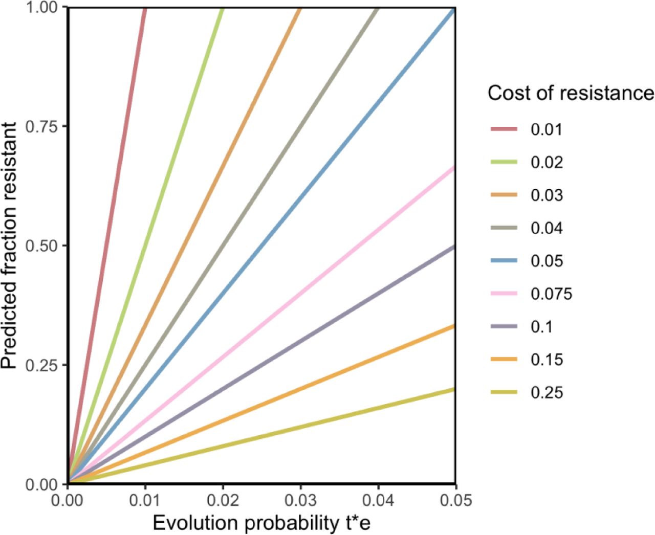
f = (t ⋅ e)/(c) , see Figure 2. This equilibrium result can explain the stability of the level of resistance (f), the linear relationship between treatment levels (through t) and the level of resistance (f), while allowing for evolution of new resistant strains to occur.

Higher levels of treatment lead to higher values of t⋅e, consistent with Key Observation 2 about drug resistance. Strains acquire resistance by mutation or through HGT. Resistant strains can be transmitted to other hosts, with an R0 that is reduced by c compared to the R0 of susceptible strains.
Genomic and phenotypic data
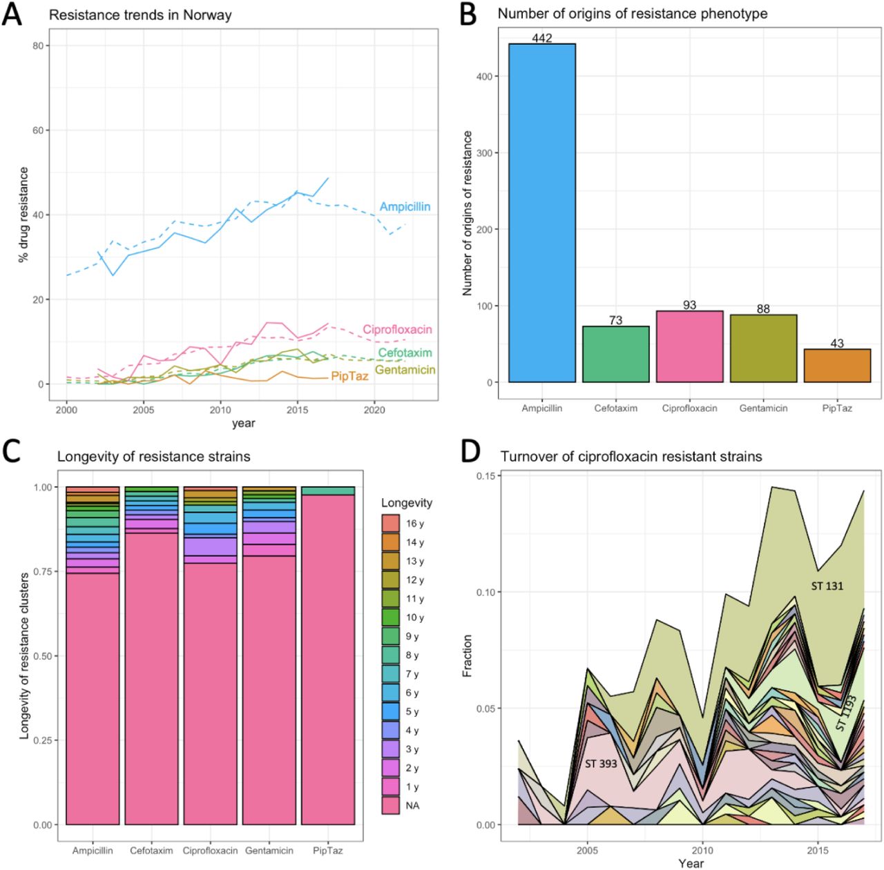
Using 16 years of publicly available data for resistance to several drugs in E. coli in Norway [28], we show that resistance acquisition is common and that most resistant strains are short-lived, which is consistent with the RAPS model. We used a dataset of E. coli genomes from bloodstream infections in Norway consisting of 3254 isolates from a surveillance program from 2002 - 2017. The fraction resistant strains in the dataset closely follows the reported fractions resistance from the European CDC surveillance atlas (see Figure 3A), which shows that even though the samples come from bloodstream infections, they are capturing important E. coli resistance dynamics in Norway.

Using the phylogenetic tree and the phenotypic resistance data provided by the authors of the original paper [28], we estimated that ampicillin resistance evolved over 400 times on the tree, and resistance to the other drugs (cefotaxime, ciprofloxacin, gentamicin and piperacillin-tazobactam) evolved between 43 and 93 times (Figure 3B) [see Methods]. Note that the big difference in the number of evolutionary origins between ampicillin and the other drugs is consistent with the fact that ampicillin is an antibiotic that is much more often prescribed than the others [20].
We found that for the five drugs we looked at, at least 75% of the strains were observed in only one year in the dataset (Figure 3C). The lifespan of individual resistant strains was estimated by determining, for each origin of resistance, in which years the resulting resistant strain was observed in the dataset. Next, we created an area plot that shows how most ciprofloxacin (quinolone) resistant strains are only seen for a short time span, but that also shows a few longer-lived strains and one resistant strain that is long-lived and reaches a high frequency (3D). While the many strains that appear and disappear again are consistent with the RAPS model, the model cannot explain the behavior of the strain that increases in frequency over several years. In fact, it is unlikely that this increase is driven by the resistance to ciprofloxacin, instead, as others have suggested, it could be that by chance the ciprofloxacin resistance mutations landed on a background with positively selected elements and are hitchhiking to high frequency [16].
In summary, our analysis of the Norwegian dataset shows that resistant strains to five different drugs evolve often, yet most resistant strains do not stay in the population for long, which is consistent with ongoing selection against resistance and with the RAPS model. Yet, there are a few long-lived resistance strains which are unexplained by the RAPS model which account for a significant portion of resistance in E. coli.
Discussion
In order to understand, predict and influence levels of drug resistance in pathogens, we need mathematical models. Here we show that a simple model with strong positive selection for drug resistance within treated hosts and mild negative (purifying) selection in the rest of the population can explain three key observations about drug resistance in a variety of pathogens (Figure 1). First, the resistance acquisition – purifying selection (RAPS) model explains the stable coexistence of resistance and susceptibility in pathogen populations. Second, it explains the positive correlation between the amount of drug used and the frequency of drug resistance (Figure 2). And finally, it recapitulates the simultaneous existence of many different strains that carry a resistance mutation or genetic element at any one time (Figure 1C).
A major strength of the RAPS model is its simplicity. It relies on only a few assumptions and doesn’t require consideration of co-infection or spatial structure of the host population. One benefit of this simplicity is that the model is more likely to be applicable to different pathogen systems. The most important assumption we make is that resistance comes with a fitness cost for the pathogen, reducing its R0 – if that is not the case, resistant strains will outcompete susceptible strains [29]. A major difference between our model and some previous models that attempt to explain stable coexistence of drug resistance and susceptibility [2,3] is that the RAPS model includes the creation and dying out of resistant strains. This can happen even when the specific genetic elements that confer resistance are stably present in the population. One reason why researchers have often chosen to ignore the creation and dying out of resistant strains is because it is assumed that drug-resistant strains are stable. However, stability at the phenotypic level doesn’t necessarily mean stability at the genetic level. New strains may evolve resistance in the same way as previous strains, even acquiring genetic elements from previous strains. The result is that the genetic element or the mutation may be stably present, but “who” carries it may always be changing (Figure 3D).
Another major strength of our model is that it makes clear and testable predictions. 1. It predicts that for a given drug, the higher levels of resistance in countries with high drug usage is due to the fact that resistance acquisition happens more often. We should therefore see more independently evolved resistant strains in countries with high levels of resistance. 2. The lifespan of resistant strains in a population should depend on the cost of the resistance for the pathogen. High-cost resistance should be associated with a shorter life span and, conversely, when resistance strains are generally short-lived this suggests that costs of resistance are high. 3. The time scale at which resistance levels change when treatment habits change should depend on the lifespans of resistant strains. Short life spans mean that a new equilibrium can be reached faster, and interventions should pay off more quickly. Intervention studies where ciprofloxacin (quinolone) use was reduced seem to indicate that this influences resistance levels in a few months [30,31]. Thanks to publicly available data, we were able to show that stability at the population level hides dynamic changes at lower levels (see Figure 3A-D). Although the resistance phenotype is present at a stable level (Figure 3A), resistance is due to many evolutionary origins (Figure 3B) and 75% of resistant strains are only present for a year (Figure 3C-D). It will be of interest to see if more granular data (e.g., monthly surveillance from a hospital) would show the waxing and waning of resistant strains. A major open question is why there are some long-lived resistance strains while most are so short-lived. Are these long-lived strains hitchhiking with other genetic elements as others have suggested [16]? Do these strains occasionally lose the resistant phenotype, as would be expected if the resistance is a costly hitchhiker?
It is of interest to see if what we know about treatment levels and drug resistance evolution probabilities roughly fits with the model. We are aware of estimates for f (fraction resistant), t (treatment probability per year) and e (probability of evolution given treatment) for quinolone drugs. We can plug in those numbers in the equilibrium equation to get an (admittedly very rough) estimate for the cost of resistance per year. In 2015, the fraction of E. coli resistant to quinolones f ≈ 10% in Norway. We also know, for Norway, that the use of quinolones is around 0.5 doses per day per 1000 people [21] . If we assume that a course of quinolones is 5 days, this translates into t ≈ 3.3% probability per year of someone taking a course of quinolones ((0.5 DDD*365 days) / (5 days per course*1000 people)*100%). A recent study estimated that the probability of resistance evolution due to a course of quinolones is e ≈ 10% [32]. Because our model proposes that f = (t ⋅ e)/(c) , we have 0.1 = 0.033 ∗ 0.1 / c, which means that the fitness cost should be around 0.033 or 3.3% per year. While we cannot currently know if this number is correct, it is encouraging to see that the number is at least of an order of magnitude that seems plausible. It would be of interest to see whether phylogenetic approaches can be used to determine if resistant strains indeed have a lower R0 compared to non-resistant strains [33,34].
If stable levels of resistance mask the ongoing appearance of new resistant strains, this may have implications for machine learning methods that are used to predict drug resistance phenotypes from genomic data. At any given year and location, a machine learning algorithm may learn to recognize certain strains responsible for much of the resistance burden in a species. Yet, over time, these resistant strains may be replaced by others, which means that we likely need to re-train such models for current and local situations [35].
Our study has several limitations. One limitation is that the model considers only resistance to a single drug and not interactions between drugs or resistances. For example, when plasmids carry multiple resistance genes, resistance to one drug can be acquired due to selection for resistance to another drug. We also assumed that treatment does not affect transmission. If treatment itself is associated with strongly reduced transmission (as is the case in HIV), then it would be useful if the model included the treatment state of hosts, where the transmission probability of hosts on treatment is significantly lower than those not on treatment [33,36]. The cost of resistance may also vary between strains and may be affected by compensatory mutations [29,37].
In conclusion, we propose a simple model that explains why drug resistance can stably co-exist with susceptible strains at levels that depend on drug usage. The model also explains why drug resistance is often present in many different strains (phylogenetic clusters, genetic backgrounds or sequence types) and predicts that resistant strains evolve and disappear again regularly. Data for resistance to several drugs in E. coli in Norway are largely consistent with these predictions, though the model does not explain why some resistant strains are seen over many years. This novel model has the potential to help us understand, predict and influence drug resistance levels and because of its simplicity, it can be readily tested in many different pathogen systems such as S. pneumoniae [2,3], S. aureus [4] and HIV [5,6]).
Data Availability
All data and code are on github: https://github.com/pleunipennings/CoexistencePaper
Methods
All code and data are available on github https://github.com/pleunipennings/CoexistencePaper.
Figure 1A European surveillance data
Quinolone resistance over time in 10 European countries.
Data were downloaded from the European Surveillance Atlas for Infectious Diseases. Link https://atlas.ecdc.europa.eu/public/index.aspx.
As health topic, we chose “Antimicrobial resistance”, as subpopulation “Escherichia coli|” and “fluoroquinolones” and as indicator “percentage resistance”. We then downloaded a csv file with data for all available years and regions (named ECDC_surveillance_data_Antimicrobial_resistance_complete_DownloadApril2024.csv in the Github repository). For Figure 1A we included the 10 most populous countries in the EU, including the United Kingdom: Germany, United Kingdom, France, Italy, Spain, Poland, Romania, Netherlands, Belgium, Czech Republic [20].
Figure 1B European surveillance data
For figure 1B, we used the percentage fluoroquinolone resistance in 2015 from the dataset described for Figure 1A, but now for the 20 most populous countries. This included in addition to the first 10: Sweden, Portugal, Greece, Hungary, Austria, Bulgaria, Denmark, Finland, Slovakia, Ireland.
For data on the use of fluoroquinolones in these countries, we downloaded data from https://www.ecdc.europa.eu/en/publications-data/antimicrobial-consumption-annual-epidemiological-report-2015 which included “Downloadable tables: Antimicrobial consumption - Annual Epidemiological Report for 2015” [21].
Figure 1CE. coli phylogenetic tree Kallonen dataset from Nouhuijs et al
The phylogenetic tree in Figure 1C was reproduced from [15]. Data presented here include only E. coli strains from phylogroup D and F. The genomes and phenotypes were described in [16]. Briefly, a core genome alignment was used to create a phylogenetic tree, then we simulated a single history of the resistance phenotype using the “simmap” function in Phytools [38,39], the simulated history is shown on the tree with resistant branches in red, susceptible branches in green and intermediate branches in green.
Figure 3A Resistance trends in Norway for five drugs
Data are from Gladstone, 2021 [28] and from the ECDC Surveillance Atlas [20].
Figure 3B Estimated number of origins of resistance to five drugs
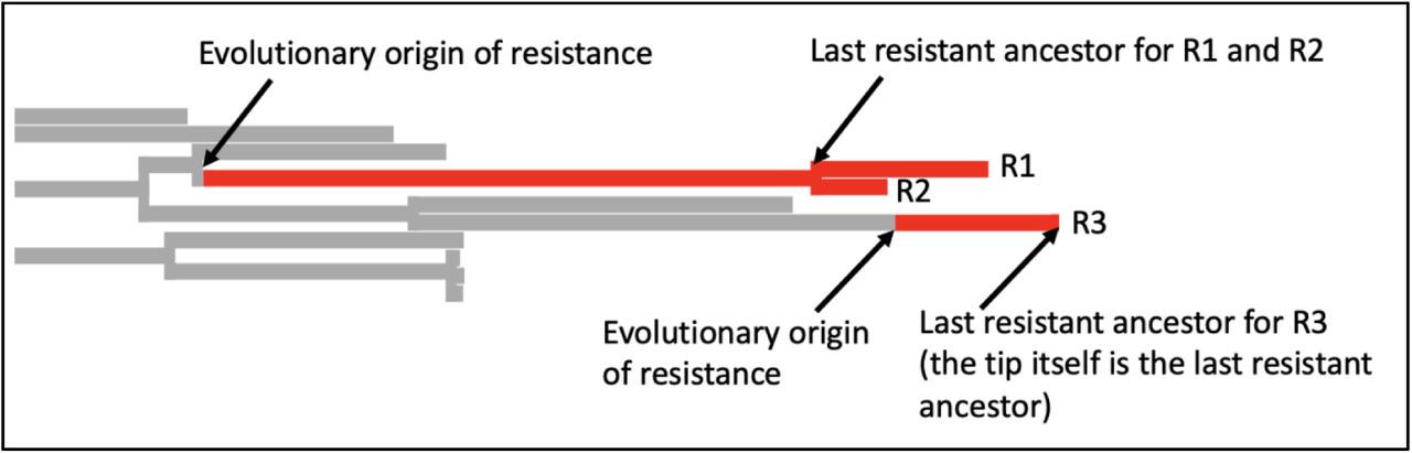
We used the tree and metadata provided by Gladstone, 2021 [28]. This dataset consists of 16 years of surveillance data including 3254 E. coli samples from bacteremia patients in Norway between 2002 and 2017. Intermediate and susceptible strains were lumped in one category. We simulated a single history of the resistance phenotype using the “simmap” stochastic character mapping function in Phytools [39] which is based on methods by [38,40]. Next, we used a custom R script to identify the last resistant ancestor for each resistant tip of the tree. If two tips share a last resistant ancestor, we assume that they are resistant due to the same evolutionary origin of resistance. This evolutionary origin may be due to a mutation, several mutations or horizontal gene transfer – our approach is based on the phenotypes, not the genotypes. Based on the simmap results, we count the number of times resistance was acquired on the tree.

In this example, there are three resistant tips. The branches are colored according to the simmap stochastic character mapping. R1 and R2 share a last resistant ancestor and are therefore assumed to be resistant due to the same evolutionary event in their history, we consider them part of the same resistant cluster or resistant strain. For R3, the last resistant ancestor is itself. It is the only member of the resistant cluster or strain.
Figure 3C Lifespans of resistant strains
Using the results from analysis described for 3B and the metadata from [28] to determine for each inferred resistance cluster for how many years it was observed in the data. For example, if R1 was a sample from 2005 and R2 was a sample from 2007, then we infer that the lifespan of this cluster was 3 years.
Acknowledgements
I am grateful for comments from and discussions with Kristin Harper, Joachim Hermisson, Sarah Cobey, Alison Feder, Nandita Garud, Oana Carja, Rasmus Nielsen, Alison Hill, Scott Roy, Brandon Ogbunu, Ruth Hershberg and the students in the SFSU CodeLab.
Footnotes
I changed the data I used to test some of the model predictions. Instead of data from the UK I now used data from Norway.
Bibliography


