
Abstract
Due to their low frequency, estimating the effect of rare variants is challenging. Here, we propose RareEffect, a method that first estimates gene or region-based heritability and then each variant effect size using an empirical Bayesian approach. Our method uses a variance component model, popular in rare variant tests, and is designed to provide two levels of effect sizes, gene/region-level and variant-level, which can provide better interpretation. To adjust for the case-control imbalance in phenotypes, our approach uses a fast implementation of the Firth bias correction. We demonstrate the accuracy and computational efficiency of our method through extensive simulations and the analysis of UK Biobank whole exome sequencing data for five continuous traits and five binary disease phenotypes. Additionally, we show that the effect sizes obtained from our model can be leveraged to improve the performance of polygenic scores.
Introduction
With the availability of extensive sequencing data in biobanks1, the study of rare variants has become more feasible than ever before. Rare variants have been identified as potential causative factors for numerous complex diseases2-8, and their exploration is crucial in unraveling the genetic risk factors of complex traits9. To identify the association between rare variants and complex traits, gene or region-based tests10,11, including the Burden test, the sequence kernel association test (SKAT)12 and its adaptive optimized version (SKAT-O)13, have been commonly used. Recently, several methods, including STAAR14, SAIGE-GENE15, and SAIGE-GENE+16 are developed to run region-based tests in biobank scale data.
To elucidate the effect of rare variants on complex diseases and traits and utilize them for risk prediction, in addition to calculating p-values for association tests, effect size estimation is required. However, estimating the effect size of rare variants remains a challenge. The low minor allele frequencies make single variant-based estimations unstable. Popular association tests like SKAT and SKAT-O are score tests, so only provide p-values. Although the Burden test approach provides a gene-burden effect size, this may not accurately reflect the true effect of rare variants in the presence of null variants and variants with opposing association directions.
To address the challenges, we introduce RareEffect, a novel method that estimates gene or region-based heritability and subsequently calculates each variant’s effect size using an empirical Bayesian approach. Utilizing a variance component model, similar to that in the SKAT test, our method offers dual-level effect size estimation, region-level and variant-level, for enhanced interpretability. Unlike the Burden approach, our model flexibly estimates effect sizes in a data-driven manner. To reduce the computational burden for estimating variance components, we implemented the Factored Spectrally Transformed Linear Mixed Models (FaST-LMM)17, which leverages the low rank of the genetic relatedness matrix. We also utilize the strategy to collapse ultra-rare variants, as used in SAIGE-GENE+, to reduce the sparsity of the genotype matrix and improve power of estimating the effect of ultra-rare variants. For binary traits, we additionally apply a fast implementation of the Firth bias reduction method to stably estimate the effect sizes.
From simulation studies, we showed that the proposed method is computationally fast and reliably estimates each gene heritability. We also showed that the proposed approach outperformed linear regression or ridge regression in terms of root mean squared error (RMSE) for estimating the individual-variant level effect sizes. From the UK Biobank (UKB) Whole Exome Sequencing (WES) data analysis of 5 quantitative traits and 5 binary disease traits, we demonstrate that exonic rare variants can explain substantial phenotypic variabilities, but the degree differs by phenotypes. We also showed that our approach has higher explanatory power in explaining the phenotype variability compared to models based on burden tests. These findings provide strong evidence for the practical utility of our method in leveraging rare variant data for risk prediction and heritability estimation.
Result
Overview of methods
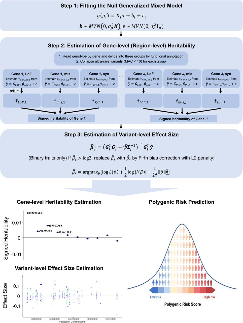
Our proposed method encompasses three steps. The overview of the method is outlined in Fig. 1 and is described in detail in the Methods section.

RareEffect encompasses three steps. In step 1, we fit a null GLMM using AI-REML approach, and obtain residuals for the subsequent steps. In step 2, we divide variants by gene and its functional annotation (LoF, missense, and synonymous). We first estimate the variance component of each group and adjust them using MoM approach. In step 3, we calculate the variant-level effect size using BLUP estimates. For binary traits, Firth bias correction is additionally applied to adjust the case-control imbalance. Through RareEffect, we provide region-level and variant-level effect sizes for enhanced interpretability and improved risk prediction performance.
In step 1, we fit a null linear or logistic mixed-effect model without genotypes to estimate the covariate effects. This step involves fitting the model using the average information restricted maximum likelihood (AI-REML)18 approach, which is utilized in the SAIGE19 and GMMAT20 framework. Residuals will be used as covariate-adjusted phenotypes in the subsequent steps.
In step 2, we model the effect of rare variants (MAF≤0.01) as random effects and estimate the variance components, and hence heritability. To mitigate the computational demands, we adopt the Factored Spectrally Transformed Linear Mixed Models (FaST-LMM)17. Given n ≫ k, FaST-LMM reduces the computation cost from O(n3) of conventional mixed model algorithm to O(nk2) where n is the number of samples in the dataset and k is the number of genetic variants in a single group (See Methods). Additionally, we leveraged the sparsity in genotypes. To incorporate the fact that genetic effects vary by functional annotations, we fit the model separately for distinct categories, and then combine them to calculate gene or region-level heritability. For whole exome analysis, we include three functional categories: (1) Loss-of-function (LoF) variants; (2) missense variants; and (3) synonymous variants. Within each category, the ultra-rare variants, defined as those with a minor allele count (MAC) of lower than 10, are collapsed into a single variant, as employed in SAIGE-GENE+16. As estimating multiple variance components due to distinct functional groups is not feasible with FaST-LMM, we marginally calculate variance component for each functional group separately, and then adjust them using method of moments (MoM) approach (See Methods).
In step 3, following the estimation of variance components, we calculate the effect size of each variant using the Best Linear Unbiased Predictor (BLUP) estimates21-24. We further estimate the prediction error variance (PEV) of the effect size estimates to assess the reliability of the variant-level effect sizes. Additionally, using the estimated PEV, we can obtain confidence intervals for each variant-level effect size. For binary traits, we implemented Firth bias correction as a subsequent step. This correction mechanism mitigates bias and rectifies abnormal estimates, especially in scenarios where the case-control ratio is imbalanced. Recognizing the imperative of scalability in large-scale biobank data analyses, we developed a fast implementation of Firth correction, which reduces computation complexity from O(MnkF) to O(nnzkF) where M is the average number of iterations for convergence of Firth corrected beta, nnz is the number of individuals with non-zero genotype, and kF denotes the number of variants that needs to be corrected (See Methods).
UK Biobank WES data analysis
We applied our method to five quantitative traits (HDL cholesterol, LDL cholesterol, triglycerides, height, body mass index (BMI)) and five binary traits (breast cancer, prostate cancer, lymphoid leukemia, type 2 diabetes, and coronary atherosclerosis) in UKB. For LDL cholesterol (LDL-C) level, we adjusted the pre-medication levels by dividing the raw LDL-C level by 0.7 for individuals on cholesterol-lowering medication25.
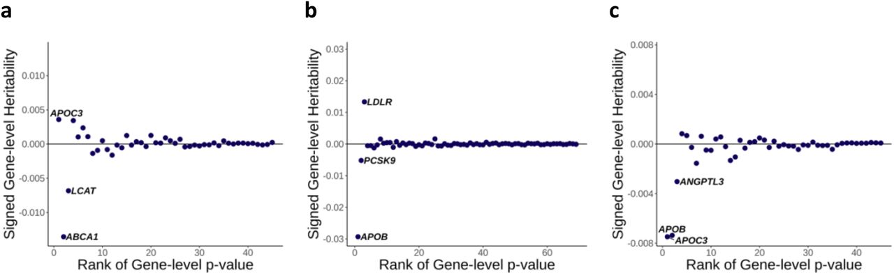
We computed gene-level effect sizes by leveraging the estimated heritability derived from the mixed effects model. Recognizing the inherent unsigned nature of heritability, we assign a sign by incorporating variant-level effect sizes of loss-of-function (LoF) variants within each gene. This allows us to discern the direction of the effect of the gene on the trait (See Methods). As expected, the gene-based association test p-values and the magnitude of the gene-level effect size showed a substantial correlation (Fig. 2 and Supplementary Figure 1). Incorporating gene-level effect size and direction on top of the gene-based association tests can add significant value to genetic analyses. For example, the signed heritability clearly shows that the impairment of APOC3 function increases HDL cholesterol (HDL-C) level but decreases triglycerides (Fig. 2(a) and 2(c)).

Signed gene-level heritability from RareEffect for (a) HDL cholesterol level, (b) LDL cholesterol level, and (c) triglycerides level. Gene-level p-values were obtained from SAIGE-GENE+, and we included genes with p-values < 2.5 × 10⁻⁶. The x-axis represents the rank order of genes based on their gene-level p-values. Lower ranks correspond to genes with more significant p-values. The y-axis shows the signed gene-level heritability for each gene. Signed heritability indicates the direction (positive or negative) and magnitude of the genetic contribution of the gene to the trait.
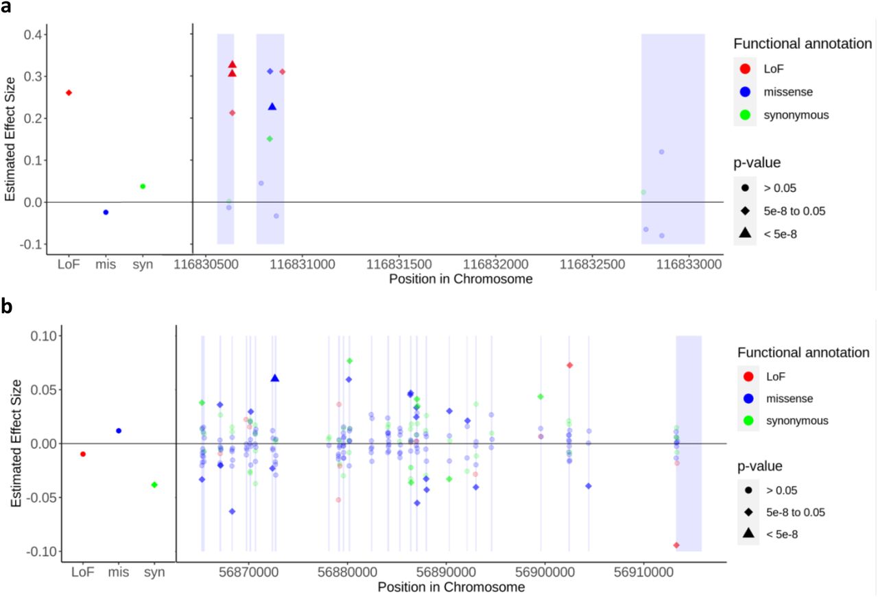
We estimated the variant-level effect sizes of exonic variants and presented two genes, APOC3 and SLC12A3, on HDL-C levels as examples (Fig. 3). As expected, variants demonstrating significant associations, in terms of p-values, also exhibited larger effect sizes. Using RareEffect, we observed that the majority of variants in APOC3 displayed positive effect sizes. The Burden and SKAT-O p-values from SAIGE-GENE+ were both highly significant (Burden p-value = 1 × 10−298 and SKAT-O p-value = 1 × 10−300). In contrast, variants in SLC12A3 exhibited both positive and negative effect sizes. Consequently, Burden p-value was not significant (Burden p-value = 0.01), but the SKAT-O p-value was significant (Burden p-value = 7 × 10⁻¹²). This distinction in the directionality of effect sizes cannot be discerned through the burden approach.

Variant-level effect size on HDL cholesterol level for (a) APOC3 and (b) SLC12A3 genes. Gene-level p-values were obtained from SAIGE-GENE+, and we included genes with p-values < 2.5 × 10⁻⁶. The left panel shows the effect size of collapsed ultra-rare variants categorized by their functional annotations: loss-of-function (LoF), missense, and synonymous, respectively. The right panel displays the variant-level effect size of rare variants. Variants are color-coded based on their functional annotation: red for LoF, blue for missense, and green for synonymous. The shapes of the points indicate the significance of the variants: circles represent p-values > 0.05, diamonds represent p-values between 5 × 10⁻⁸ and 0.05, and triangles represent p-values < 5 × 10⁻⁸. Single-variant p-values were obtained from SAIGE, while the p-values of collapsed variants were derived from linear regression by regressing  on each collapsed variant. The exon region is shaded.
We extended our analyses to estimate polygenic risk scores using rare variants with effect sizes estimated from RareEffect (PRSRE). The UK Biobank data were randomly split into training and test sets (ratio = 8:2), and PRSRE was constructed using the genes with p-values < 2.5 × 10⁻⁶ from SAIGE-GENE+ in the training set (See Methods). We included top 10 genes when the number of genes with p-values < 2.5 × 10⁻⁶ is smaller than 10. We further integrated these PRSRE with PRS derived from common variants (PRScommon) to evaluate the practical utility of our approach. When combining the PRS from common and rare variants, we constructed a composite score, a linear combination of PRS from common and rare variants. We evaluated the predictive performance in terms of R2. Our methods consistently exhibited superior prediction accuracy for all tested quantitative traits, compared to a comparative approach that relied on per-allele effect sizes derived from burden tests (Fig. 4, Supplementary Table 1, and Supplementary Figure 2).

Coefficient of determination (R2) of the risk prediction models for (a) HDL cholesterol level, (b) LDL cholesterol level, and (c) Triglycerides level. We evaluated the R2 of five models using: (1) PRSburden only, (2) PRSRE only, (3) PRScommon only, (4) composite score, (5) PRScommon + PRSRE + PRSburden by five subgroups: (1) all samples, (2) samples with top/bottom 10% PRS, (3) samples with top/bottom 5% PRS, (4) samples with top/bottom 1% PRS, and (5) samples with top/bottom 0.5% PRS. The black vertical lines represent the 95% confidence interval of the R2 estimates.
The improvement became particularly pronounced when predicting lipid phenotypes among individuals deemed at high risk. For instance, when predicting HDL and LDL cholesterol levels, PRSRE achieved R2 of 0.4737 and 0.6287 when restricting individuals with top/bottom 0.5% in terms of PRSRE. When the composite score was used for risk prediction, R2 were 0.6237 and 0.6645 when restricted top/bottom 0.5% individuals. In contrast, common variants only PRS model had lower R2 (0.5417 for HDL and 0.5823 for LDL) for top/bottom 0.5% individuals. Notably, the sub-groups identified as high-risk by PRScommon and PRSRE were substantially distinct (Supplementary Figure 3), underscoring the complementary nature of rare variants in detecting individuals at elevated disease risk. Additionally, we observed that our model showed higher predictability compared to the Burden approach which showed R2 of 0.3683 and 0.2262 for HDL and LDL with top/bottom 0.5% in terms of PRS using burden score (PRSburden), respectively.
Our method exhibited marginally lower predictive performance for binary traits, as measured by AUC, compared to the burden approach. We observed that for chosen binary traits, there were fewer genes associated with the trait, and their signals appeared weaker when contrasted with tested continuous traits. Nonetheless, our method offers potential benefits, as it can enhance predictability by combining PRSRE with PRScommon and PRSburden, which yielded better results. For instance, in the case of lymphoid leukemia, when evaluating individuals in the top/bottom 0.5% based on common PRS, the PRScommon + PRSRE + PRSburden approach exhibited an AUC of 0.8649, whereas the PRScommon + PRSburden approach demonstrated an AUC of 0.8559, with the common-only approach yielding an AUC of 0.8559.
We further examined the relationship between phenotype outliers and the PRS in identifying individuals at high risk for common diseases26. We first defined the phenotype outliers as individuals with phenotype value exceeding a certain z-score cutoff and calculated the proportion of individuals with high PRS among phenotype outliers. Specifically, for LDL cholesterol levels, PRSRE successfully pinpointed individuals at phenotypic extremes, who exhibited a tenfold higher likelihood of possessing a PRSRE falling within 0.1st percentile compared to the baseline population (Supplementary Figure 4). PRSRE and PRScommon utilize distinct set of variants and show minimal correlation (Supplementary Table 2). Therefore, integrating these models into a unified framework enables the identification of a significantly larger cohort at high risk than achievable through PRScommon alone.
Simulation study
To assess the predictive accuracy of our method, we conducted extensive simulations under diverse scenarios (see Methods) for both binary and quantitative traits. To mimic real data, we utilized actual genotypes from the UKB dataset, specifically the array-genotyped data for common variants (MAF≥0.01) and the UKB WES data for rare variants (MAF≤0.01).
We compared the performance of our method against other existing approaches such as linear regression, which is used for standard single-variant association test, or ridge regression in terms of RMSE. For quantitative traits, our method consistently demonstrated a lower RMSE of 0.1703 on average, outperforming the comparative methods which showed RMSE of 0.1770 (ridge regression) to 0.1881 (linear regression) (Supplementary Table 3) when estimating the effect size. For binary traits, our method also exhibited lower predictive error particularly in scenarios of low disease prevalence compared to ridge regression (Supplementary Table 4). Conversely, ridge regression showed marginally reduced error compared to our method in instances of high disease prevalence; however, the difference in accuracy remains modest.
Computation and memory cost
Analyzing 166,960 samples from the UKB WES data to estimate the effect size of the DOCK6 gene, which contains 4,114 rare variants, we observed that the computation time for RareEffect with a simulated phenotype was approximately 90% lower than that of ridge regression. Specifically, RareEffect completed the analysis in 4.2 seconds, compared to 44.6 seconds for ridge regression (Supplementary Figure 5). The memory usage for RareEffect during the analysis was 1.14GB for DOCK6 gene (Supplementary Figure 6). For binary traits, an additional step of performing Firth bias correction is required. We observed that the normal Firth bias correction process took 708 seconds to analyze a gene with 250 variants (after collapsing) across 342,409 individuals. However, by implementing our fast version of Firth correction, the computation time was dramatically reduced to 2.9 seconds (Supplementary Figure 7).
Discussion
Our study introduces a novel method aimed at estimating the effect size of rare variants and can be extended to estimate gene-level effect size by employing a two-stage framework of generalized linear mixed models. By leveraging the variant-level effect size estimates obtained through our approach, we can examine the collective impact of rare variants within a gene and quantify their contribution to the overall heritability of complex traits.
In order to obtain accurate estimates for effect sizes while optimizing computational efficiency, we employed several techniques in our analysis. First, we utilized the FaST-LMM17 algorithm to expedite computation and reduce memory usage. FaST-LMM leverages the spectral decomposition of the genetic relatedness matrix, allowing for efficient calculation of the variance component in mixed models. Second, we implemented the optimized version of Firth bias correction by utilizing the sparsity of genotype matrix and skipping the computation of hat matrix at every iteration. Third, we employed a collapsing strategy that reduces the sparsity of the data, similar to the approach employed in SAIGE-GENE+. These algorithmic approaches significantly accelerate the estimation process and enhance computational scalability, particularly when dealing with large-scale datasets and complex genetic analyses involving rare variants.
Beyond its immediate applications in effect size estimation, our proposed method offers significant potential for enhancing polygenic risk prediction models. Traditionally, these models have relied on common variants, often neglecting the valuable insights provided by rare variants. Our analysis reveals that the correlation between PRSRE and phenotype values in the general population is not substantial (Supplementary Figure 8). However, we demonstrate that the RareEffect method effectively identifies individuals with high genetic risk. By incorporating our approach, we can substantially improve the predictive accuracy and precision of polygenic risk scores.
AI-based methods27,28 have been developed to enhance the pathogenicity prediction of rare variants. Although these approaches help to identify effect sizes of pathogenic variants and can be used for risk prediction, they may not be as effective for identifying beneficial or gain-of-function variants. Additionally, the performance of these methods can be limited when applied to non-protein-altering variants. Our approach can accommodate the predictively pathogenic variants identified by AI-based models by forming them into a separate category, thereby enhancing performance.
Our study, however, is not without limitations. While RareEffect demonstrates comparable or superior performance in estimating the effect size for simulated binary phenotypes, our evaluation revealed only marginal enhancements in predictive performance, as measured by the area under the curve (AUC), compared to the traditional common PRS across tested disease phenotypes. This could be attributed to the trait’s reliance on a limited number of ultra-rare variants, which our method collapses into super-variants, thereby complicating the estimation of variant-level effect sizes for true causal variants. Despite its efficacy in effect size estimation, RareEffect’s ability to improve prediction accuracy remains constrained, highlighting a potential area for future refinement and investigation for risk prediction of binary traits. Additionally, it is important to note that RareEffect is based on BLUP estimate, characterized by shrinkage properties, leading to biased estimates of effect sizes. However, despite this bias, RareEffect provides more stable estimates compared to unbiased methods like linear regression, which tend to be unstable for rare variant analysis due to the low allele frequency inherent in such variants.
In summary, our results demonstrate that incorporating information from rare variants enables the accurate estimation of gene-level and variant-level effect sizes, as well as the identification of high-risk individuals who might remain undetected by conventional polygenic risk scores (PRS) methods relying on common variants.
Method
Generalized linear mixed model
We denote the phenotype of the ith individual using yi for both quantitative and binary traits in a study with sample size n. X represents the n × (p + 1) vector with p covariates including the intercept and Gj is the n × k matrix representing the minor allele counts for k rare variants in gene or region j. The generalized linear mixed model (GLMM) can be expressed as:
 where μ is the mean phenotype,
  is the random effect, and K is an n × n genetic relatedness matrix (GRM). And g is the link function which is an identity function for quantitative traits with error term
  and a logit function for binary traits. The parameter α is a (p + 1) × 1 vector of fixed effect coefficients and βj is a k × 1 vector of the random genetic effect.
Fitting the null generalized mixed model (step 1)
We used the average information restricted maximum likelihood (AI-REML) algorithm to fit the null GLMM (i.e., H0: βj = 0) as in SAIGE step 1.
Estimation of the gene-level (region-level) heritability (step 2)
We estimate the effect size of rare variants using the following linear mixed model:
 where
where  for quantitative traits,
  , a working residual from iteratively reweighted least squares (IRWLS) for binary traits, and
  is the mean phenotype for individual i, which can be obtained from step 1. When obtaining Gj, as in SAIGE-GENE+, we collapsed ultra-rare variants with minor allele count (MAC) ≤ 10 by each gene and functional group to reduce the sparsity. We further implemented an option to collapse all loss-of-function (LoF) rare variants into a single column, irrespective of their minor allele count, adopting the burden approach. This approach is predicated on the assumption that all rare LoF variants share a common effect size and direction. For binary traits, when we use working residuals, the variance of
  differs by individual, so we cannot apply the optimization technique of FaST-LMM. Therefore, we divide both sides by the square root of variance of
  to make the variance be the same across individuals. We estimate the effect size using the modified model, for binary traits:
 where
where  .
.
In this model, the prior distribution of βj are assumed to follow MVN(0, τΣ), and the noise ϵ is assumed to follow MVN(0, ψIn) for quantitative traits, while we assume  follows MVN(0, ψIn) for binary traits. When there is no prior knowledge of the correlation within β, Σ is set to be an identity matrix. But in general, Σ does not have to be an identity or a diagonal matrix.
To estimate the variance component parameters (τ, ψ), we use factored spectrally transformed linear mixed models (FaST-LMM) algorithm. Let  be an n × k genotype matrix of the region with
  for quantitative traits and
  for binary traits. The variance of
  (quantitative traits) or
  (binary traits) can be written as

Traditional approaches to estimate the variance components require either calculating inverse matrix or conducting spectral decomposition of the n × n matrix  , so the time complexity is of O(n3). In contrast, FaST-LMM algorithm uses the fact that
  has rank at most k, so to reduce the computation complexity. Suppose
  is an n × k matrix where L is a Cholesky factor of Σ. Then
  . FaST-LMM carries out singular value decomposition on Z and calculate likelihood for (τ, ψ). With given n ≫ k, calculation of Z and its singular value decomposition requires only O(nk2) of time complexity. And we further improved the computation efficiency utilizing the sparsity of Z29. In biobank-scale data, n is in the hundreds of thousands, and k is in the tens to hundreds on average which means n ≫ k.
Using the above optimization technique, we estimate the variance components by each group. Consider one group (LoF, missense or synonymous) in a single gene j in the model:

We first marginally estimate the maximum-likelihood estimator (MLE) of variance components τLoF,j, τmis,j, and τsyn,j. As the marginal estimates do not account for LD among variants in different groups, we adjust the estimates using method of moments (MoM) approaches30. The MoM estimator can be obtained by solving the following linear system:
 where T is a 3 × 3 matrix for joint estimation or a scalar (1 × 1 matrix) for marginal estimation with entries
  where k, l ∈ {1, 2, 3} for joint estimation. b is a 3-vector for joint estimation or a scalar for marginal estimation with entries
  , c is a 3-vector for joint estimation or a scalar for marginal estimation with entries
  , and
, and  where (τ1, τ2, τ3) denotes (τLoF,j, τmis,j, τsyn,j) for a single gene j, respectively.
After estimating the marginal and joint MoM estimator of variance components, we adjust the MLE of the marginal variance components by:
 where i ∈ {LoF, mis, syn}. The MoM estimator of the variance component was not directly utilized in our study since the MoM estimator could yield negative variance components. In cases of the variance component estimated by the MoM is negative, we used marginal variance component without adjustment. Both MoM and likelihood-based approaches exhibited the similar trends of variance components (Supplementary Figure 9). Additionally, we assume that the variance explained by rare variants in a single gene is negligibly small compared to the total variance of
  , therefore,
 .
.
We estimated the heritability from rare variants of gene j using these adjusted variance components. In a joint model,
 where
where  .
.
Therefore,

Subsequently, the heritability from rare variants of gene j can be denoted as:

Additionally, to determine the direction of the gene-level effect, we obtained the sign of the linear combination of the effect sizes of loss-of-function variants in a gene, weighted by their MAFs:

This measure gives the information of the magnitude of genetic effects from rare variants in a single gene and its direction of effects.
Estimation of the variant-level effect size (step 3)
The effect sizes at variant-level resolution are estimated using the adjusted variance components in the previous step by:
 for each gene or region.
We further estimated the prediction error variance (PEV) by:
 for each gene or region. Using this PEV, we can obtain confidence intervals for effect sizes.
For binary traits, the Firth bias correction31 is a more accurate method to estimate SNP effect sizes32-34, particularly in cases marked by a significant case-control imbalance. We incorporate this correction into our analytical framework. Additionally, we introduce an L2 penalty term to account for the prior distribution of β. The Firth corrected effect estimates can be calculated numerically by optimizing the following objective function:

where L denotes the likelihood function and I is the Fisher information.
To improve computational efficiency, we developed the fast implementation of Firth bias correction. First, we compute the hat matrix,  , only once rather than recalculating it at each iteration, assuming that the iterative weights (W) change slowly as a function of the mean μi 20,35. We compared, using both simulation and real data, the difference in effect size estimates between computing the hat matrix once and computing it at each iteration. Our findings indicate minimal differences in the effect size estimates (Supplementary Figure 10). Given that Firth correction is applied to each variant, we iterate the hat matrix calculation for kF times, where kF represents the number of variants that need to be corrected. This strategy results in a reduction in the computational complexity with Firth correction from O(MnkF)to O(nkF), where M is the average number of iterations needed for Firth corrected effect size convergence. Second, we extend Firth correction to accommodate sparse genotype matrices. Specifically, we restrict our computations to individuals with non-zero genotypes when determining the score and Fisher information. This further reduces the time complexity of the Firth correction, now at O(nnzkF), where nnz denotes the number of individuals with non-zero genotype. Considering that we are estimating the effect size of rare variants with MAF < 0.01, we observed that nnz < 0.01n which implies that leveraging sparsity makes the estimation of effect sizes more than 100 times faster compared to a non-sparse approach.
We note that Firth correction is used when the absolute value of estimated effect size  surpasses a predefined threshold. In this study, we used threshold of log 2 ≈ 0.693 for simulation studies and real data analysis.
Rare-variant PRS calculation
We further calculated polygenic risk scores using the variant-level effect sizes of rare variants (PRSRE) in genes with gene-level p-value from SAIGE-GENE+ lower than 2.5 × 10⁻⁶. PRSRE of individual i can be calculated as:
 where J denotes a set of genes with gene-level p-value lower than 2.5 × 10⁻⁶. Additionally, we combined these PRSRE with PRScommon only. We applied PRS-CS36 to obtain the variant-level weights for the calculation the PRScommon. We compared the predictive performance of the PRSRE to PRSburden. PRSburden were obtained in two different ways: (1) collapsing all rare variants into one super-variant regardless of the functionality of the variants and (2) collapsing rare variants by functionality of the variants (LoF, missense, and synonymous). After collapsing, we fitted the following linear model to estimate the per-allele effect sizes:

The burden PRS are also calculated as a linear combination of per-allele effect sizes and the collapsed genotypes of each individual.
We compared the predictive performance in terms of R2 for quantitative traits, and the area under receiver operating characteristic curve (AUROC) for binary traits of the following linear models:
 where PRScomposite is a linear combination of PRScommon and PRSRE with weights trained from the training set.
UK Biobank data analysis
In this study, we used WES data of 393,247 White British participants in the UK Biobank. The UK Biobank is a UK-based prospective cohort of ∼500,000 individuals aged 40 to 69 at enrollment. We split the train and test data 8:2 randomly for the PRS evaluation. We applied quality control (QC) procedures prior to the analysis. We first removed redundant samples and individuals with sex mismatch or sex chromosome aneuploidy. Additionally, we further removed variants with a missingness rate across individuals > 0.1, HWE p-value < 10−15, and monomorphic variants. We generated group files, which define the list of variants in genes and its functional annotation, by using the loss-of-function transcript effect estimator (LOFTEE)37. We regarded a variant as loss-of-function (LoF) only in case of it is labeled as a high-confidence (HC) LoF variant, and variants with low-confidence (LC) were regarded as missense variants.
Using the data after QC, we applied our method to five quantitative traits (HDL cholesterol, LDL cholesterol, triglycerides, height, and body mass index) and five binary traits (breast cancer, prostate cancer, lymphoid leukemia, type 2 diabetes, and coronary atherosclerosis). We defined the disease by mapping ICD-10 codes to Phecodes using the PheWAS R package38.
Simulation study
To generate outcome phenotypes, we used the following model for quantitative and binary traits:
 where Xi1 and Xi2 are covariates, and Gi,common and Gi,rare are genotype vectors of common variants and rare variants of i th individual, respectively. The intercept α for binary traits is determined by the disease prevalence. The covariates Xi1 and Xi2 were simulated from Bernoulli(0.5) and N(0, 1), respectively. For common variant effect, we randomly selected L =30,000 LD-pruned common variants with MAF > 1%, and assumed that the effect size of single common variant follows
  . We selected 10 causal genes in UKB WES 200k data for generation of phenotypes. We used eight different scenarios regarding rare variants: (1) proportion of causal variants, (2) effect size of causal variants, and (3) direction of effect within a single gene. For the proportion of causal variants, we assumed (1) 20% of LoF, 10% of missense, and 2% of synonymous variants, or (2) 30% of LoF, 10% of missense, and 2% of synonymous variants among rare variants that are not ultra-rare are causal. For ultra-rare variants, we assumed that the proportion of causal variants are three times higher than the non-ultra-rare variants, that is, (1) 60% of LoF, 30% of missense, and 6% of synonymous ultra-rare variants, or (2) 90% of LoF, 30% of missense, and 6% of synonymous ultra-rare variants are causal. Regarding the effect size of causal variants, we assumed that the absolute effect sizes of causal variants are (1) |0.5 log10 MAF| for LoF variants, and |0.25log10 MAF| for missense and synonymous variants, or (2) |0.3 log10 MAF | for LoF variants, and |0.15log10 MAF| for missense and synonymous variants. We further assumed that the effect directions are (1) the same among all causal variants in a single gene, or (2) same for 100% of LoF, 80% of missense, and 50% of synonymous variants, while remaining variants have the opposite direction of effect. For eight combinations of scenarios, we repeated the simulation for 100 times.
Computation cost evaluation
We evaluated the computation time and memory usage using simulated data as described above, comprising 166,960 individuals of White British ancestry from the UKB WES 200k dataset. Additionally, we examined computation time and memory usage across subsets with sample sizes of 10k, 30k, 50k, and 100k. For each generative scenario, we reported the mean of 5 attempts for computation times and memory usage, comparing them with multiple linear regression, simple linear regression (as in GWAS), and ridge regression. The evaluation for linear regression and ridge regression was done using lm and glm functions in R, respectively.
Data Availability
The analysis results for 5 quantitative and 5 binary phenotypes of UKB WES data analysis results are available at: https://storage.googleapis.com/leelabsg/RareEffect/RareEffect_effect_size.zip (variant-level effect size) and https://storage.googleapis.com/leelabsg/RareEffect/RareEffect_h2.zip (gene-level signed heritability).
Data availability
The analysis results for 5 quantitative and 5 binary phenotypes of UKB WES data analysis results are available at: https://storage.googleapis.com/leelabsg/RareEffect/RareEffect_effect_size.zip (variant-level effect size) and https://storage.googleapis.com/leelabsg/RareEffect/RareEffect_h2.zip (gene-level signed heritability).
Code availability
RareEffect is implemented as a part of SAIGE software, which is an open-source R package, available at https://github.com/saigegit/SAIGE. RareEffect is available in SAIGE version 1.3.7 or higher.
Author Contribution
K.N. and S.L. designed experiments. K.N. performed experiments and analyzed the UKB WES data. K.N. and S.L. implemented the software with input from W.Z.. M.K. and B.M. provided helpful advice. K.N. and S.L. wrote the manuscript with input from all co-authors.
Supplementary Figures
Estimated signed heritability for 10 tested traits
Predictive performance for 10 tested traits
Relationship between common PRS (PRScommon) and RareEffect PRS (PRSRE)
Enrichment of high-risk individuals in terms of RareEffect PRS (PRSRE), common variant PRS (PRScommon) and composite score in phenotype outliers
Computation time of RareEffect, linear regression, and ridge regression
Memory Usage of RareEffect by number of variants
Computation time of the fast implementation Firth bias correction and the normal Firth correction
Relationship between RareEffect PRS (PRSRE) and phenotype values
Comparison of estimated variance components between RareEffect and MoM estimator
Comparison of estimated effect size between computing the hat matrix at every iteration and only once in Firth bias correction
Supplementary Tables
Predictive performance for 10 tested phenotypes in UK Biobank
Pearson correlation between PRScommon and PRSRE
Predictive performance (RMSE) for simulated continuous data by scenario
Predictive performance (RMSE) for simulated binary data by scenario
Acknowledgements
This research was supported by the Brain Pool Plus (BP+) Program through the National Research Foundation of Korea (NRF) funded by the Ministry of Science and ICT (2020H1D3A2A03100666) and the grants funded by the Ministry of Food and Drug Safety, Republic of Korea (Grant Number: 23212MFDS202). This research was conducted using the UK Biobank Resource under application number 45227.


