
Abstract
In this article, we formulate and analyze a mathematical model for the coinfection of HBV and COVID-19 that incorporates the effects of Brownian and Lévi noise. We studied the dynamics and effects of these diseases in a given population. First, we establish the basic reproduction number of the disease-free equilibrium point of the stochastic model by means of a suitable Lyapunov function. Additionally, we provided sufficient conditions for the stability of the model around the disease-free equilibrium points. Finally, using a few simulation studies, we demonstrate our theoretical results. In particularly, we derived threshold values for HBV only  , COVID-19 only,
  , and coinfection
  for the stochastic model around disease-free equilibrium point. Next, the conditions for stability in the stochastic sense for HBV only, COVID-19 only submodels, and the full model are established. Furthermore, we devote our concentrated attention to sufficient conditions for extinction and persistence using each of these reproductive numbers. Finally, by using the Euler–Murayama scheme, we demonstrate the dynamics of the coinfection by means of numerical simulations.
1 Introduction
Both Coronavirus Disease 2019 (COVID-19) and Hepatitis B virus (HBV) infections remain major public health threats [4]. COVID-19 is caused by Severe Acute Respiratory Syndrome Corona virus 2 (SARS-CoV-2) and affect the functionality of the respiratory system. It is spread from one person to another by coming into direct contact with respiratory droplets from an infected individual. It can also spread by touching surfaces contaminated with the virus and then touching the face. On the other hand, HBV disease is caused by the hepatitis B virus and is associated with serious liver infection, leading to liver malfunction, including cirrhosis, liver fibrosis, and hepatocellular carcinoma. Both COVID-19 and HBV are life-threatening diseases that have been declared global health problems [18]. For example, [32] reported that more than 3 billion people are infected with HBV globally. An estimated 7 million COVID-19 deaths and 700 million infections have been reported since December 2019 [18]. These statistics demonstrate how devastating HBV and COVID-19 diseases are worldwide. Presently, global efforts have been made to develop and distribute COVID-19 vaccines, aiming to reduce severe illness, hospitalizations, and deaths.
Over the years, mathematical models have provided frameworks for explaining transmission dynamics and for making necessary interventions for several infectious diseases; see, e.g. [2, 11, 28, 5, 7, 16]. Several models of COVID-19, HBV and other infectious disease transmission dynamics have been developed in the literature.
The transmission dynamics of COVID-19, HBV, and other diseases have been extensively studied, mostly in isolation. Both deterministic and stochastic models have been developed to understand the spread of these diseases [13, 11, 9]. In [11], the authors deemed the susceptible-exposed-infectious-recovered (SEIR) model introduced by [34] to describe the transmission dynamics and forecast the national and global spread of COVID-19 disease to be simplistic and largely unrealistic because it excluded the relapse from recovered class to susceptible class. Like [34], authors including [22, 30] also made an assumption of no relapse from the recovered to the susceptible class, an assumption that is critiqued in [28]. [26] examine the extinction and persistence for a HBV only model and also conducted simulations on the model.
Amidst inconclusive findings from clinical studies on whether one disease increases the severity of another disease in the event of coinfection (see e.g. in [4, 29]), there has been a spike in interest for both clinical and theoretical scientific research on disease coinfections in recent times. The theoretical study of coinfection through mathematical modelling will be valuable to shaping our understanding of transmission dynamics of these diseases. A number of studies that have been done on co-dynamics of COVID-19 including Dengue [23], cholera [10], malaria, [20, 1, 21, 3, 19] and co-dynamics s TB, see, e.g. [24, 14]. [29] employed a deterministic model and examined the effects of optimal control strategies on the Covid-19, HBV coinfection transmission. On the other hand, [8] examined COVID-19 and HBV coinfection by employing Gaussian noise to explain the perturbation in observed data for the COVID-19 and Malaria coinfection model. Stochastic coinfection models are very scarce in literature, and more so for COVID-19 and HBV Stochastic coinfection models. While mathematical models, see, e.g., [17, 28], have been proposed to describe the dynamics of diseases including COVID-19 and HBV, there is a dearth in studies imprint the effect stochastic perturbations on COVID-19-HBV coinfection. In this paper, we employ both Gaussian noise and Non-Gaussian noise to explain the noise in the Coinfection of COVID -19 and HBV in the presence of COVID-19 Vaccination, and determine conditions for extinction and persistence for the coinfection model.
Stochastic coinfection SIRS models unlike classic or deterministic SIRS models, incorporate the effects of random fluctuations in the transmission dynamics of disease and recovery rates, as well as the possibility of coinfection by different diseases. In [35, 15], the authors formulated techniques for examining existence, uniqueness and persistence of solution. Understanding and analysing the dynamics of infectious illness transmission in both humans and animals can benefit from mathematical modelling. The persistence or extinction of the diseases depends on several factors, such as the basic reproduction numbers, the coinfection rates, and the stochastic perturbations; hence, determining the conditions for the persistence or extinction of the diseases is a cumbersome task. One of the methods proposed to analyze the persistence or extinction of stochastic coinfection SIRS models is the use of Lyapunov functions, which are scalar functions that measure the distance from an equilibrium point [33]. For example, [33] employed Lyapunov functions to show that if the basic reproduction numbers of both diseases are less than one, then the disease-free equilibrium is globally asymptotically stable for a stochastic coinfection SIRS model with nonlinear incidence rates and cross-immunity effects. In this paper we develop condition for extinction and persistence for coinfection model.
In this article, we will formulate a mathematical model which builds on (2) of [8] by firstly assuming relapse to susceptible state. The new model includes COVID-19 vaccination state, and also assume the presence of both standard random fluctuation and massive disturbances which arise due to sudden environmental shocks in the transmission dynamics. The novel coinfection model will open up some new avenues for further research in stochastic modelling dynamics of coinfection of diseases. Specifically, our study seeks to investigate the following objectives:
To develop a compartmental model for explaining the transmission dynamics of HBV-COVID-19 coinfection.
To establish the Invariance and Positivity of the stochastic system for coinfection Model.
To determine the basic Reproductive number for Stochastic HBV Only, COVID-19 Only and Coinfection models respectively.
To determine conditions for stability at Disease Free Equilibrium for Stochastic HBV Only, COVID-19 Only and coinfection models respectively using Brownian Noise and Poisson Lévi Noise.
To present numerical simulations and discussions of the model.
The rest of the paper is organised as follows; Section 2 discusses the Mathematical Model and the underlying assumptions. In Section 3, we analyze the COVID-19, and HBV sub-models as well as the Coinfection model. Section 4 is devoted to discussing the numerical method and numerical simulation of the model. Finally, we present the conclusion in Section 5.
2 Mathematical Model Formulation
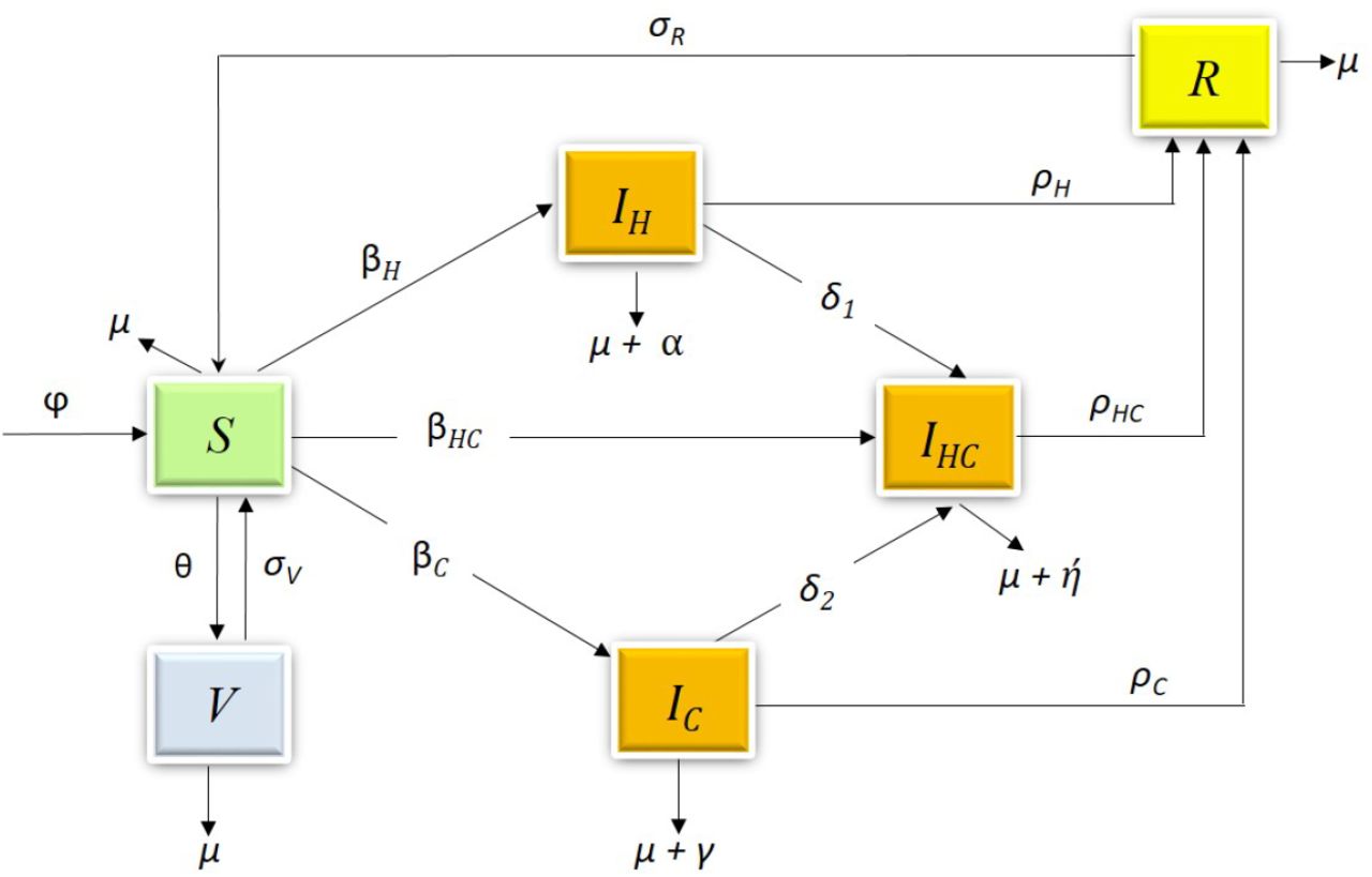
In this section, we consider a stochastic compartmental mathematical model that uses differential equations, see Figure 1.

Compartmental diagram for the COVID-19 Hepatitis B coinfection cohort.
The sub-populations of the human population at time t, denoted by N (t), include susceptible individuals S(t), COVID-19 vaccinated individuals V (t), COVID-19 infected individuals IC(t), Hepatitis-B infected individuals IH (t), individuals infected with both COVID-19 and Hepatitis-B IHC(t), and recovered individuals R(t).
We will consider the following assumptions;
(A1) The total human population (N (t)) is a sum of all the different compartments, i.e.

(A2) Covid-19 Vaccination wears off after some period of time. (A3) There is relapse to susceptible state,
(A4) There is no vertical transmission.
 with initial conditions S(0) > 0, IC(0) ≥0, IH (0) ≥ 0, IHC(0) ≥0, R(0) ≥0, V (0) ≥ 0. βC, βH are the effective contact rate for COVID-19, and HBV respectively.
Two popular ways to introduce stochastic factors into epidemic models are: (i) to assume some small and standard random fluctuation, (ii) to assume massive disturbances caused by sudden environmental shocks. The first, is described by Gaussian white noise while the second is described by the Lévy noise. It is assumed that fluctuations in the environment will manifest mainly as fluctuations in the parameter β, i.e. β → β + ϵidBi(t), (i = 1, 2, …, 6), where dBi(t) is a one dimensional standard Brownian motion with Bi(0) = 0, and ϵi is the intensity of the white noise. Also a multiplicative noise is considered in our model, as random term depends on the state space, e.g. [8]. The Lévy jump process, thus, is divided into linear drift term, Brownian motion and compensated Poisson Process. The stochastic model of the system (2) takes the following form:
 where dBi(t) is independent of
  . 𝒩 is a Poisson counting measure with compensating martingale
  and characteristic measure v on a measurable subset 𝒰 ∈ (0, ∞) where v(𝒰) ≤ ∞ and Ψi : 𝒰 → ℜ (i = 1, 2, 3, 4, 5, 6) denotes the effects of random jumps and is bounded and continuous. It is assumed that v is a Levy measure so that
  . We note that S(t−), IH (t−), IC(t−), IHC(t−), R(t−), V (t−) denote the left limits of S(t), IH (t), IC(t), IHC(t), R(t), V (t) respectively.
The following definitions are necessary for the analysis of the stochastic model.
(Itô-Lévi [26]). First, set  . Suppose a complete probability space (Ω, F, Ft ≥ 0, P) with filtration Ft ≥ 0, which satisfies the usual conditions. Bi(t) is defined on this probability space.
We assume an Itô -Lévi process, X(t) ∈ ℜ+, of the form
 where, F : ℜn × ℜ+ × S → ℜn, G : ℜn × ℜ+ × S → ℜn, and Ψ : ℜn × ℜ+ × S × Y → ℜn are measurable functions and X(t−) denotes the left limit of X(t). F (X(t), t) represents the linear drift term, G(X(t), t) the Brownian noise,
  (dt, du) represents the compensated Poisson random measure, and Ψ(X, t, u) represents the intensity of jumps. It is assumed that the condition
(Itô-Lévi Formula [26]). We consider the process X expressed by (4) and let 𝒱 ∈ C2,1(ℜn × ℜ+ × S; ℜ+) such that 𝒴 ≡ 𝒱(t, X(t)). Then, 𝒴(t) is again an Itô-Lévi process and

Which is the representation of generalized Itô’s formula with jumps.

To gain insights into the underlying mechanisms that drive the spread of infectious diseases to identify the long-term behaviour of disease transmission we conduct qualitative analysis of the stochastic model (3).
3 Qualitative Analysis of Model
In this section, we present the Positivity of the Solution to (3), determine the Reproductive Number for Single Disease Models and Coinfection model, determine the conditions for Local and Global equilibrium for COVID-19 only, HBV only, and for Coinfection model. Further we determine the conditions for Extinction and Persistence for all three models.
3.1 Positivity of Model
A first step is to determine the positivity of solution to the stochastic system (3) as a negative state will not be biologically meaningful. We will show the positivity of the first equation in(3).
Let ((S(t), IH (t), …, V (t)) be a solution of system (3), given initial values ((S(0), IH (0), …, V (0)) ∈ Ω, where Ω ∈ ℜ+, then limt→∞ S(t) ≥ 0, limt→∞ IH (t) ≥ 0, …, limt→∞ V (t) ≥ 0.
Proof. Let us consider (3). By eliminating terms and rearrangement, we obtain
 where r = βH IH (t)+βCIC(t)+βHCIHC(t) − (µ+θ). Next, we take a function g(t, S(t)) = ln(t, S(t)) and apply Itô’s formula to get,

Combining (6) and (7), solving for S(t) and taking the limit we obtain,

Hence S(t) is positive definite. Similarly, limt→∞ IH (t) ≥ 0, limt→∞ IC(t) ≥ 0, limt→∞ IHC(t) ≥ 0, limt→∞ R(t) ≥ 0, limt→∞ V (t) ≥ 0.
3.2 Invariant Region of Stochastic COVID-19 and Hepatitis B Coinfection Model
An investigation of the invariant region of the model will help us determine the set of states for which the disease will eventually either persist or die out infinitely.
Let N(t) be the population of system (3), given initial values N (0) > 0, and  , then
  , and (S(t), IH (t), …, V (t)) ∈ Ω.
Proof. By adding and simplifying terms in (3) and choosing ϵ = max(ϵi) we obtain;

Applying (5) we have,

We let  . The complementary solution to (3)) was obtained as

Next, we determine the particular solution of (8) and obtain the general solution of (8) as

We then find the limt→∞ of the general equation of (8) and apply comparison to obtain

3.3 Disease Free Equilibrium Point
We consider the first equation of (3). For disease free equilibrium, we have IC(t) = 0, R(t) = 0, and let  , solve for S(t), and apply comparison to obtain,

Since 0 < ϵ1(dB1) + ∫ 𝒰 Ψ1(u) < m <∞, where m is a positive constant, the final inequality is obtained by comparison. Hence, the disease free equilibrium is given by

3.4 Reproductive Number of COVID-19 only Model
Given D.F.E. point  , the Reproductive Number of COVID-19 only model
  .
.
Proof. Applying Itô-Lévi formula to the COVID-19 infected class of (3), we obtain

Considering initial infections F and secondary infections V, we determine the basic reproduction number by means of the next generation matrix as follows

Taking the spectral radius of F V −1, i.e., ρ(F V −1), we obtain,

3.4.1 Local Stability of COVID-19 Only Model
If  , then for any initial values of
  , IC(t) satisfies
Proof. By integrating both sides of (11) and evaluating at disease free-equilibrium point point, we have,
 where
where
 are a martingales given
  . Dividing through by t and taking lim supt→∞ of both sides, we get,

The final inequality holds if  , which implies,
 .
.
3.4.2 Global Stability of COVID-19 Only Model
If  , then E0C is globally asymptotically stable in Ω.
Proof. We consider the Lyapunov function,
 For
For  and Q =(γ + μ + ρC)
 since
since  . Hence L1 is globally stable in the domain Ω.
3.5 Basic Reproduction Number for HBV Model
We consider only HBV transmission in human. The model of the system is given as (3).
Given D.F.E. point  then the Reproductive Number of HBV only Model
  .
.
Proof. Applying Itô-Lévi formula to the HBV infected class of (3), we obtain,

Considering initial infections F and secondary infections V, we determine the basic reproduction number by means of the next generation matrix as follows;

Taking the spectral radius of F V −1, i.e., ρ(F V −1), we obtain,

3.5.1 Local Stability of HBV Only Model
If  , then for any initial values of
  satisfies
  .
.
Proof. We integrate both sides of (12) and evaluate at D.F.E. point to obtain,

Next, we divide through by t, find lim sup → ∞ and apply the strong law of Martingales as follows,
 which completes the proof.
  as (α + µ + ρH) > 0, which implies,
  where
where  , and
, and  are a martingales given
  .
.
3.5.2 Global Stability of HBV Only Model
If  , then E0H is globally asymptotically stable in Ω
Proof. We consider the Lyapunov function L2,

For  ,and P = (α+ μ+ ρH).
 hence L2 is globally stable in the domain Ω.
3.6 Reproductive Number of Coinfection Model
Given D.F.E. point  , the Reproductive Number of Coinfection
  .
.
Proof. Applying Itô-Lévi formula to the Coinfected equation of (3), we obtain,

Considering initial infections F and secondary infections V, and since 

Taking the spectral radius of FV −1, i.e.,  we obtain,

3.6.1 Local Stability of Disease Free Equilibrium point in the Coinfection Model
If  , then for any initial values of (S(0), IH (0), IC(0), IHC(0), R(0), V (0)) ∈ ℜ6, IHC(t) satisfies
  .
.
Proof. Integrating (14), eliminating terms, choosing constants, and setting G = (η + µ + ρHC) yields,

Next, we divide through by t, find lim sup and apply the strong law of Martingales as follows,

The final inequality holds if  as (η + µ + ρC) > 0, which implies,
  where
where  , and
, and  are a martingales given
  .
.
3.6.2 Global Stability of Coinfection Model
If  , then E0HC is globally asymptotically stable in Ω
Proof. We consider the Lyapunov function, Net we differential and employ comparision to determine conditions for Global Stability of Coinfection.
 hence L3 is globally stable in the domain Ω.
3.7 Extinction of HBV-COVID-19 Coinfection disease
Next, we determine conditions under which the disease will eventually die out in the population with a probability of one. In this section we study the conditions of extinction for the coinfection model.
[8] We define  , and
, and  .
.
[25] Let (S(t), IC(t), IH (t), IHC(t), R(t), V (t)) be the positive solution of system(4) with given initial condition  , Let also X(t) be the positive solution of equation (4) with given initial condition given condition X(0) = N (0) = S(0) + IC(0) + IH (0) + IHC(0) + R(0) + V (0) ∈ ℜ+. Then

- ,and


Let (S(t), IH (t), …, V (t)) be the solution of (3) with initial values (S(0), IH (0), …, V (0) ∈ Ω), the coinfection disease of model (3) goes extinct almost surely (limt→∞ IHC(t) = 0) a.s if one of the following assumptions holds:
- and ,
- and ,
- .


Proof. By integrating (3), dividing by t, adding terms, followed by some algebraic manipulations we obtain the following equations:

 where
where

Next, we integrate both sides (14). Since  we get,

We divide through (17) by t. Next we substituting (15) and (16) into (17) we obtain,


Next, we find lim supt→∞ and apply a Lemma 2 and Lemma 1 to obtain following results,

 hence
hence

Similarly, we can prove  when
when  , and
, and  when
when  .
.
3.8 Persistence in mean
Persistence of a disease means that the disease will remain endemic in the population with positive probability. We study the disease persistence for the system reported in (3) and derive that the disease persists under certain some conditions.

[6] Set g ∈ ℂ [[0, ∞] × Ω, (0, ∞)], assume that there exist ξ0, ξ > 0 such that
 such that G ∈ (ℂ[[0, ∞] × Ω, (0, ∞)]) satisfying
  . Then
  .
.
Let (S(t), IH (t), IC(t), IHC(t), R(t), V (t)) be a solution of system (3) with initial values (S(0), IH (0), IC(0), IHC(0), R(0), V (0)) ∈ Ω.
If
and , the disease IH persists in mean. In addition, IH holds
If
, max (and ) < 1, then the disease IC is persistent in mean. In addition, IC satisfies


Proof. We begin with the first statement of the theorem. By rearranging terms in (15), we get:

Next, we integrate both sides of (12), and eliminate terms to obtain,

We divide (24) by t, substitute (23) into (24), and find lim inft→+∞ to get,

Then, by Lemma 2 and since  , we conclude,
 which concludes the proof. Next we prove the persistence in mean for COVID-19. Let us integrate both sides of (11), and then eliminate terms to obtain,

We divide (25) by t, substitute (23) into (25), and find lim inft→+∞ to get,

Then, by Lemma 2 and since  , we conclude,

Finally in a similar way, we can prove persistence for coinfection of diseases;

4 Numerical Results
In this section, we employ a standard numerical procedure In this section, we employ a standard numerical procedure to obtain numerical simulation results for the HBV-only, COVID-19-only, and HBV-COVID-19 coinfection models. The objective here is to verify the theoretical results obtained earlier in this paper. The parameter values used along with their sources are displayed in Table 2. A few values were assumed. As we sought to verify theoretical results, we selected initial values of S(0) = 3000, IH (0) = 10, IC(0) = 10, IHC(0) = 10, R(0) = 0, V (0) = 40 The Euler-Maruyana scheme [12] was employed in conducting the numerical simulations for all models. The results from numerical simulation for HBV only, COVID-19 only and Confection model are presented in Figures 2 - 8.

Solution for HBV Only Model.
4.1 Hepatitis B Virus Only Model
By using fixed values of all parameters shown in Table 2 we plot the curves representing the dynamics of the susceptible, infectious, and recovered classes in the HBV-only model (3). The graphs of the compartments are presented in Figure 2 reveal. From the parameter values in Table 2, we obtained our basic reproduction numbers  .
.
We observe initially, from Figure 2 that as number of infectious population increase in time, the susceptible population decrease. However, in the long run, the solution curves for both the susceptible and infective compartments behave like decreasing functions and approach a fixed point. A decrease in the number of susceptible individuals occurred within a relatively short period of the epidemic, after which there was no marked change over time. On the other hand, the decline in the number of infective compartments tends to increase but eventually declines to a fixed point. Similarly, the recovered class also approach a fixed point in the long run. In other words, all compartments will reach to the respective endemic fixed point of model (3) within a finite time and in long run.
The numerical outcomes verifies the theorem statement that when  , then the disease free equilibrium is locally and globally asymptotically stable. The impact of various parameter on the transmission dynamics of HBV is explored. Numerical results are presented in Figure 3 and Figure 4. We proceeded by first investigating the effects of effective contact rate on population of infected individuals. This was done using selected values of effective contact rate (βH = 0.001, 0.002, 0.003), while all remaining parameter values of the model were held constant. From figure 3, we observe that as values of contact rate increases, there is an increased possibility for the population to be infected by HBV, and vice versa.

HBV Infection with varied effective contact rate.

Recoveries with varied effective recovery rate.
Next, we investigated the effects of recovery rate on population of Recovered individuals (R(t)). Similarly, we held all other parameters constant, and selected varied recovery rate (ρH = 0.05, 0.06, 0.07) for this investigation. We observe Figure 4, that more individuals recover with increasing value in ρH, thus, the reducing the number of infectious individuals. From this we can conclude that by treating the infectious individuals the infected population goes to recovered state and HBV is eliminated from the community.
4.2 COVID-19 Only Model
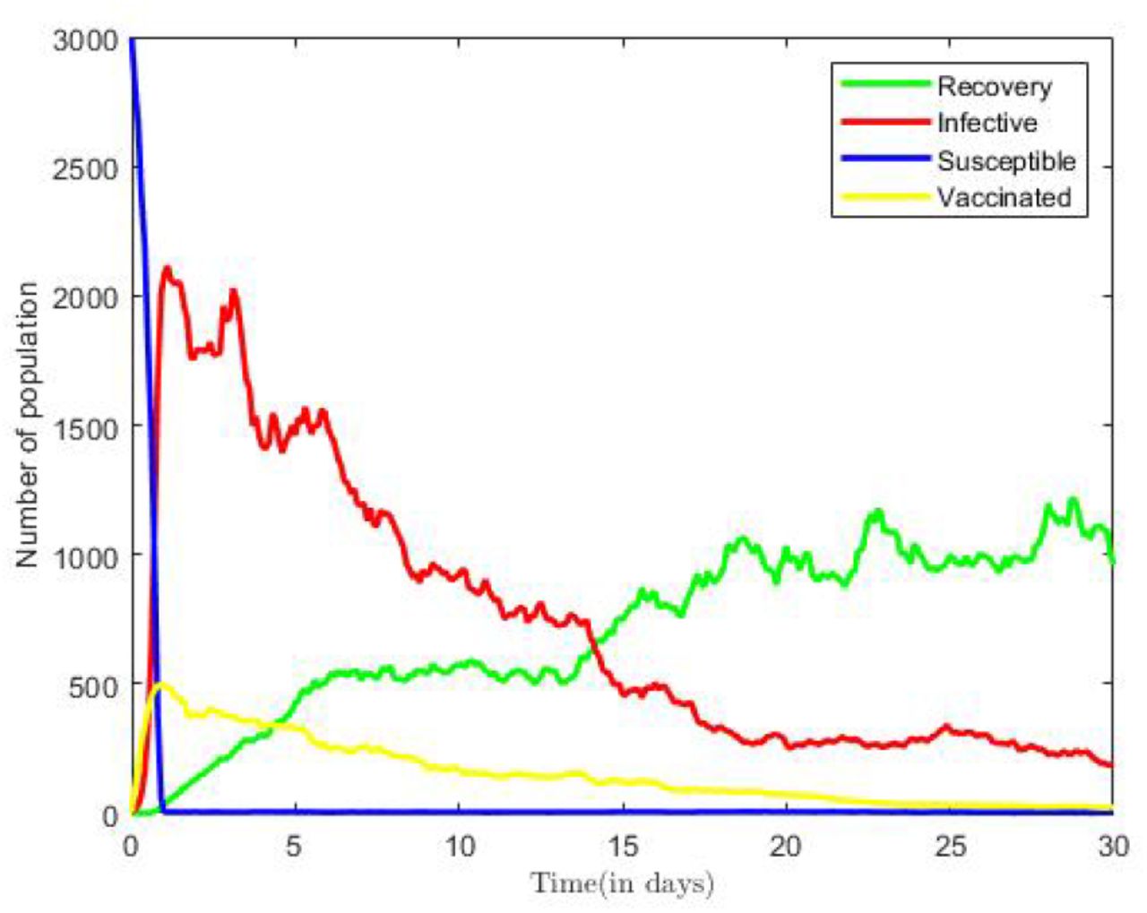
In Figure 5 simulation results representing the dynamics of Susceptible, Infectious, Vaccinated and Recovered classes in the COVID-19 only model of(3) are displayed. Figure 5 is plotted using combination of all compartments and by taking fixed values of parameters in Table 2. We observe initially, from Figure 5 that as number of infectious population increase in time, susceptible population sharply decrease. However, in the long run, the solution curves for both Susceptible and infective compartments behave like decreasing functions and approach reach to a fixed point. The decline in the number of infective compartment occurs during the after the twentieth time step of the epidemic, after which there is no remarkable change over time, but for fluctuations around the deterministic solution.

Numerical Solution for COVID-19 Only Model.
Similarly, the remaining classes, the vaccinated, and recovered populations also approach fix points in the long run. Thus, all compartments will reach to the respective endemic fixed point of the COVID-19 only model in (3) within a finite time and in long run.
The numerical outcomes verifies the theorem’ statement that when  , then the disease free equilibrium is locally and globally asymptotically stable.
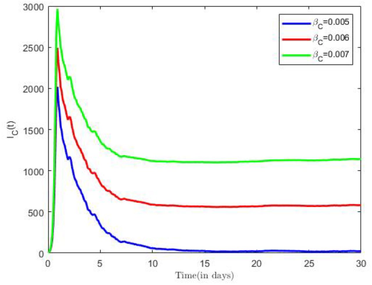
The impact of various parameter on the transmission dynamics of COVID-19 was explored. Numerical results are presented in Figure 6 and Figure 7. We proceeded by first investigating the effects of effective contact rate on population of infected individuals. This was done using selected values of effective contact rate (βC = 0.005, 0.006, 0.007), while all remaining parameter values of the model were held constant. Figure 6, shows that as the contact rate increases, the probability that the population will be infected by diseases increases, and vice versa.

COVID-19 Infection for different effective contact rates.

COVID-19 recoveries for different treatment rates.
Next, we examine the effects of recovery rate on population of COVID-19 recoveries RC(t). Again, while we held all other parameters constant, we used various recovery rate (ρC = 0.3, 0.4, 0.5). We observe in Figure 7, that more individuals recover with increasing value in ρHC, thus, the reducing the number of COVID-19 infections in the population.
4.3 Coinfection Model
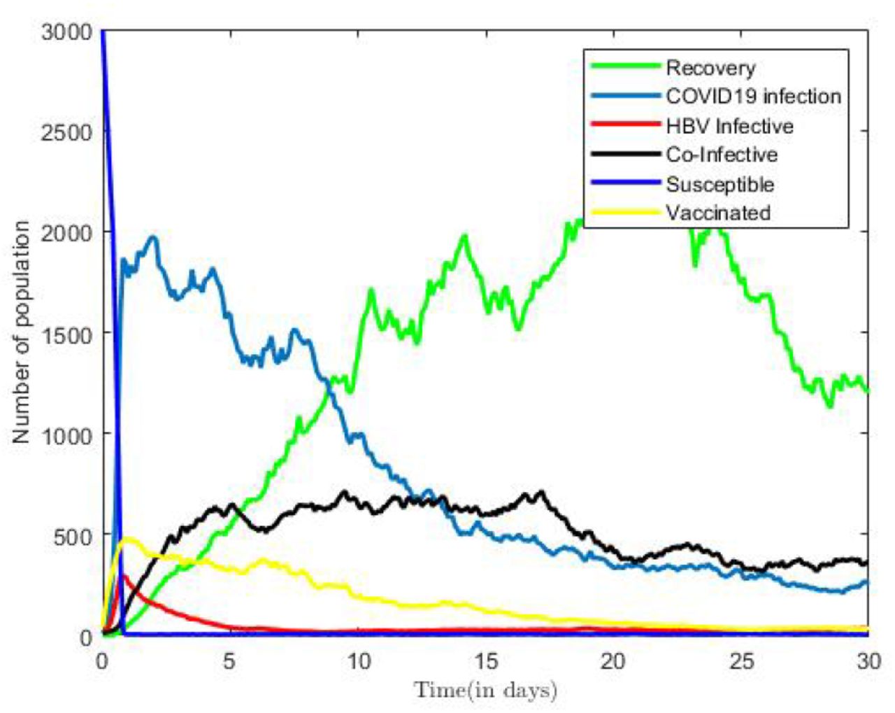
Figure 8 reveals that the curves representing the dynamics of Susceptible, Infectious, Vaccinated and Recovered classes in the coinfection model (3). Figure 8 is plotted using fixed values of all parameters from Table 2 we obtained our basic reproduction numbers  .
.

Numerical Solution for coInfection Model.
We observe initially, from Figure 8 that as number of infectious population increase in time, susceptible population will decrease, however, in the long run, the solution curves for Susceptible and infective compartments IC, IH, and IHC behave like decreasing functions and approach reach to a fixed point over time, but for oscillation around their deterministic path due to the presence of the noise.
Similarly, the all remaining classes either decrease to zero or also approach to the fixed points in the long run. In other words, all compartments will reach to the respective endemic fixed point of model (3) within a finite time and in long run. The numerical outcomes verifies Theory 10 which states that when  , then the disease free equilibrium is locally and globally asymptotically stable.
The impact of various parameter on the transmission dynamics of COVID-19 -HBV coinfection is explored. Numerical results are presented in Figure 9 and Figure 10. We proceed by first investigating the effects of effective contact rate on population of infected individuals. This was done using selected values of effective contact rate (βHC = 0.001, 0.002, 0.003), while all remaining parameter values of the model were held constant. From figure 9, we observe that as values of contact rate increases, there is an increased chance for the population to be infected by both diseases, and vice versa.

Coinfection for different effective contact rates.

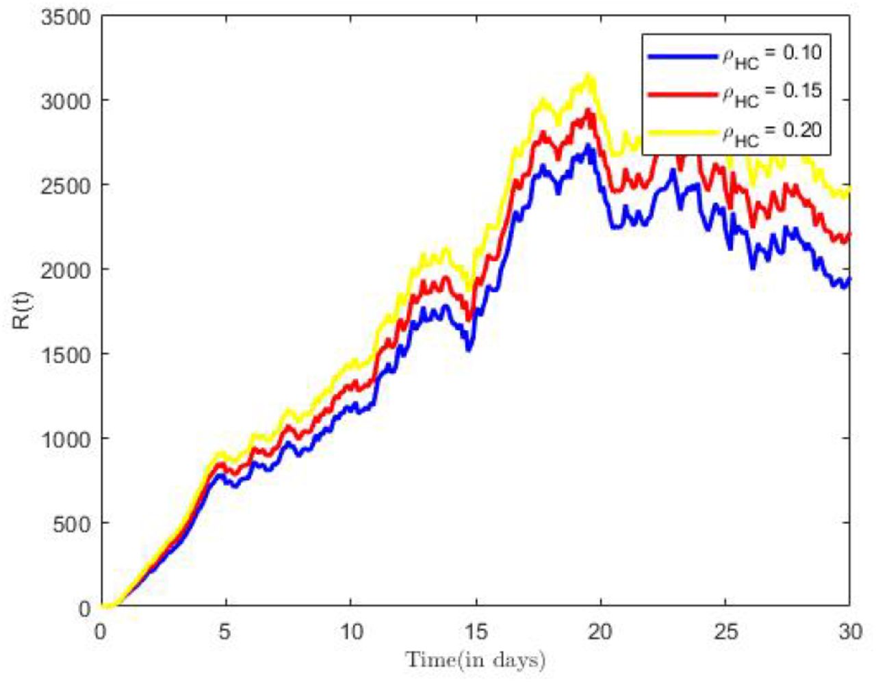
Coinfection recoveries for different treatment rates.
Next, we examine the effects of recovery rate on population of Coinfected recoveries RHC(t). Again, while we held all other parameters constant, we made use of varied recovery rate (ρHC = 0.1, 0.15, 0.2). We observe in Figure 10, that more individuals recover with increasing value in ρHC, thus, the reducing the number of coinfectious in the population.
5 Conclusion
The majority of issues in the real world are not deterministic. Because of its proximity to ambient sounds, the stochastic models allow us to model epidemic diseases in a more realistic manner. In this paper, two distinct diseases were used to study a stochastically perturbed SIRS-type model. Emphasis was given to explaining the effect of small fluctuations and perturbations due to sudden environmental shocks in the coinfection transmission dynamics, hence, the inclusion of the white noise and the Lévy noise. To determine the conditions for the local asymptotic stability of the equilibria, we first computed the reproductive number and the equilibria for the underlying stochastic model (3). Furthermore, the conditions of extinction and persistence of HBV only, COVID-19 only, and coinfection model we investigated, and it was shown that persistence for all models were dependent on the intensity of the white noise and the values of epidemic parameters involved in disease transmission.
Additionally, we demonstrated the influence of different parameters on the infectious compartments and demonstrated a broad variety of simulation results for all three stochastic models.
Data Availability
All data produced in the present work are contained in the manuscript
Footnotes
This version of the manuscript has been revised to update the following: i) Number of Authors ii) definition 1 and 2 iii) R_{0C}, R_{0H}, R_{0HC} notations in Theorem 12 iv) inclusion of two new citations.
References


