
Summary
Advancing genomic medicine relies on our ability to assess the phenotypic impacts of rare germline variants, which remains challenging even in highly sequenced monogenic disease genes. Here, we evaluate the use of population sequencing data from the UK Biobank to identify variants which alter disease risk, focusing on familial hypercholesterolemia (FH), hereditary breast and ovarian cancer syndrome (HBOC), and Lynch syndrome (CRC). We model evidence of pathogenicity from population data at the variant level, and demonstrate that odds ratios generated from population cohort data can significantly separate ClinVar pathogenic and benign variants in FH genes (p = 4.5x10⁻¹⁹), HBOC genes (p = 2.5x10-39), and CRC genes (p = 7.6x10⁻¹⁶). Next, to make use of this information in variant assessment, we calibrate population-based odds ratios (ACMG/AMP PS4) at the gene level, and find that they reach ‘strong’ or ‘very strong’ evidence of pathogenicity in 8 of 11 genes, as well as in aggregate. Among participants with a rare variant in these 8 genes, 4.3% (N = 2,456) have a Variant of Uncertain Significance (VUS) or variant not yet observed in ClinVar with strong population evidence of pathogenicity that could inform variant interpretation for a related disorder. In three genes with functional assays, we combine this population evidence with computational, contextual, and experimental evidence. Notably, 12.4% of LDLR VUS seen in participants have sufficient evidence to be classified as pathogenic. This method offers a scalable approach to integrate evidence of pathogenicity from population data.
Highlights
Uses population data to identify rare coding variants which increase risk of clinically actionable phenotypes.
Population-based disease odds ratios accurately distinguish ClinVar pathogenic and benign variants.
Calibrates odds ratios at the gene level to identify their strength of evidence for variant classification.
Combines various evidence types to reclassify a substantial fraction of variants of uncertain significance.
Introduction
Advancing genomic medicine relies on our ability to identify variants with sufficient certainty that they can be labeled ‘pathogenic’ or ‘benign’.1 Diagnostic testing has identified many pathogenic variants which increase disease risk, providing valuable insight into the molecular basis of inherited disorders.2 However, even in established disease genes like LDLR, BRCA1, and MSH2, most variants have insufficient evidence to reach a clinical classification, and are consequently classified as ‘Variants of Uncertain Significance’ (VUS).3,4 While many of these variants may substantially increase disease risk, this prognostic information cannot be communicated to patients or providers when following current clinical guidelines.5 This translational gap collectively prevents many patients from benefiting from genomic medicine, including optimized surveillance and therapeutic options.4
To standardize the information used in variant assessment, the American College of Medical Genetics and Genomics and the Association for Molecular Pathology (ACMG/AMP) sequence variant interpretation (SVI) guidelines systematically weigh and combine evidence of pathogenicity or benignity for a variant. These guidelines describe various forms of evidence (e.g., population, functional, computational, or contextual evidence) and assign strength levels to each type (supporting, moderate, strong, very strong), based on the certainty of each form of evidence. Importantly, no single source of evidence alone is considered sufficient to classify a variant as pathogenic. At the population level, when a variant is significantly enriched in disease cases over controls, it is considered ‘strong’ evidence of pathogenicity (ACMG/AMP PS4 criterion).6
Given that many damaging variants in disease genes are rare in practice, population evidence of pathogenicity has most often been derived from probands from clinical cases, research studies, or co-segregation of a variant with disease within families. Some ClinGen expert panels have defined specialized interpretation criteria for population evidence for specific genes and phenotypes. These include odds ratios (e.g., a variant with odds ratio ≥ 5.0 and lower 95% confidence bound ≥ 1, often considered ‘strong’ evidence of pathogenicity), or the number of probands, which can correspond to different strengths of evidence for a phenotype (e.g., 2-5 distinct familial hypercholesterolemia cases provide ‘supporting’ evidence of variant pathogenicity in LDLR).2,7 Recent work has evaluated the extent to which odds ratios can be used to provide evidence in support of pathogenicity, but this approach has not yet been measured or calibrated in population cohorts at the gene or phenotype level.8
Dramatic increases in biobank size now provide statistical power to detect a broader spectrum of variant effect sizes, particularly in disorders and endophenotypes which are more common or which are widely measured in population cohorts.9 Notably, endophenotypic effect sizes have been shown to discriminate between variants which are known to be pathogenic or benign in monogenic susceptibility genes, generally with larger effects.10 However, this information has yet to be generalized across a broader set of dichotomous phenotypes or calibrated for use with existing clinical guidelines, which has precluded its use in variant assessment.
Here, we draw on population case data at scale from the UK Biobank to identify variants which are enriched in a range of disorders, including familial hypercholesterolemia (FH; LDLR, APOB, PCSK9), hereditary breast and ovarian cancer syndrome (HBOC; BRCA1, BRCA2, CHEK2, ATM), and Lynch syndrome (CRC; MSH2, MSH6, MLH1, PMS2). Specifically, we model enrichment of disease using odds ratios for each phenotype based on case data at the variant level. We then align this evidence of pathogenicity within the ACMG/AMP SVI diagnostic framework by systematically calibrating the strength of evidence provided by variant odds ratios in each gene, enabling its use in clinical translation. Finally, we combine this information with well-calibrated computational and functional evidence to identify the scale of VUSs that could potentially be re-classified. By extracting and aligning population evidence in an automated manner, this framework represents a powerful step forward toward eliminating VUS.
Results
Population characteristics
To calculate variant-level odds ratios, we draw on 469,803 participants in the UK Biobank with available whole exome sequencing data. After individuals with multiple relevant variants or missing phenotype data were removed (as described in Methods), we considered 440,431 individuals for FH analysis, 250,266 individuals for HBOC analysis (excluding males), and 468,654 individuals for CRC analysis. Summary statistics for these populations are provided in Table 1A. After quality control, we observed 3,377 variants in FH genes (LDLR, APOB, PCSK9), 3,799 variants in HBOC genes (BRCA1, BRCA2, CHEK2, ATM), and 2,510 variants in CRC genes (MSH2, MSH6, MLH1, PMS2) where each variant had at least one participant in the aforementioned sets. Variant counts at the gene level are reported in Table 1B.
The number of individuals considered in our analysis of variants in FH genes, HBOC genes, and CRC genes, along with sex, age, and phenotype prevalence.
The number of variants considered in each gene analyzed.
Population-based odds ratios separate pathogenic and benign variants with high accuracy
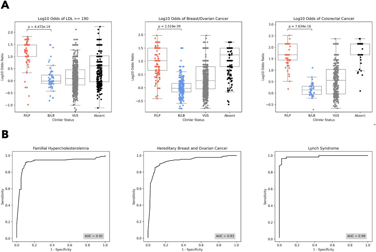
Within FH genes, ClinVar P/LP variants had a median odds ratio of 30.3 [IQR: 10.1 - 30.3] while ClinVar B/LB variants had a median odds ratio of 1.0 [0.8 - 1.7], within HBOC genes, ClinVar P/LP variants had a median odds ratio of 10.5 [4.5 - 31.5] while ClinVar B/LB variants had a median odds ratio of 1.0 [0.7 - 1.5], and within CRC genes, ClinVar P/LP variants had a median odds ratio of 46.9 [27.6 - 140.7] while ClinVar B/LB variants had a median odds ratio of 1.4 [0.9 - 2.0] (Figure 1A). For all phenotypes, population-based odds ratios significantly separated pathogenic and benign variants (Mann-Whitney U p = 4.5x10⁻¹⁹ for FH genes, 2.5x10-39 for HBOC genes, and 7.6x10⁻¹⁶ for CRC genes). At the gene level, odds ratios significantly separated pathogenic and benign variants in all genes except APOB (p = 0.17) and PCSK9 (p = 0.07), as expected based on a putative gain of function mechanisms in these genes, as well as in CHEK2 and PMS2, where there were no benign variants available (Supplementary Figure 1).

[A] The distribution of log10 odds ratios by ClinVar status (from left to right) in FH genes, HBOC genes, and CRC genes. For all three phenotypes, odds ratios separate ClinVar pathogenic (P/LP) and benign (B/LB) variants (p = 4.5x10⁻¹⁹ for FH, p = 2.5x10-39 for HBOC, and p = 7.6x10⁻¹⁶ for CRC). [B] ROC curves for classification of ClinVar pathogenic and benign variants using the population odds ratio of each phenotype for FH genes, HBOC genes, and CRC genes.
Next, we show that odds ratios can be used to classify pathogenic and benign variants with high specificity and sensitivity. Specifically, we find AUC=0.92 in FH genes, 0.93 in HBOC genes, and 0.99 in CRC genes (Figure 1B). At the gene level, AUC ranged between 0.90 and 1.00 in all genes except APOB (0.33), CHEK2 (no benign variants available), and PMS2 (no benign variants available) (Supplementary Figure 2). Taking the odds ratio thresholds at which specificity and sensitivity are maximized (most upper left point on ROC curves, which can also be interpreted as the point at which global LR+ is maximized), we find optimal odds ratio thresholds for classification at the phenotype and gene level. These thresholds vary by phenotype and gene, and are reported in Supplementary Table 3.
Systematically defining evidence thresholds for population-based odds ratios via calibration
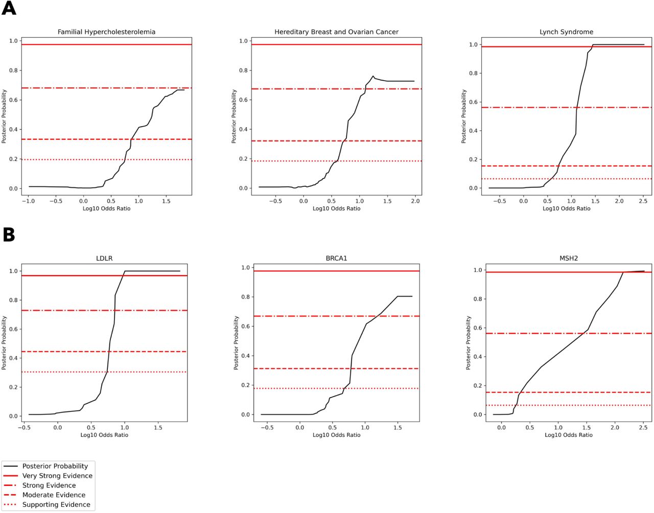
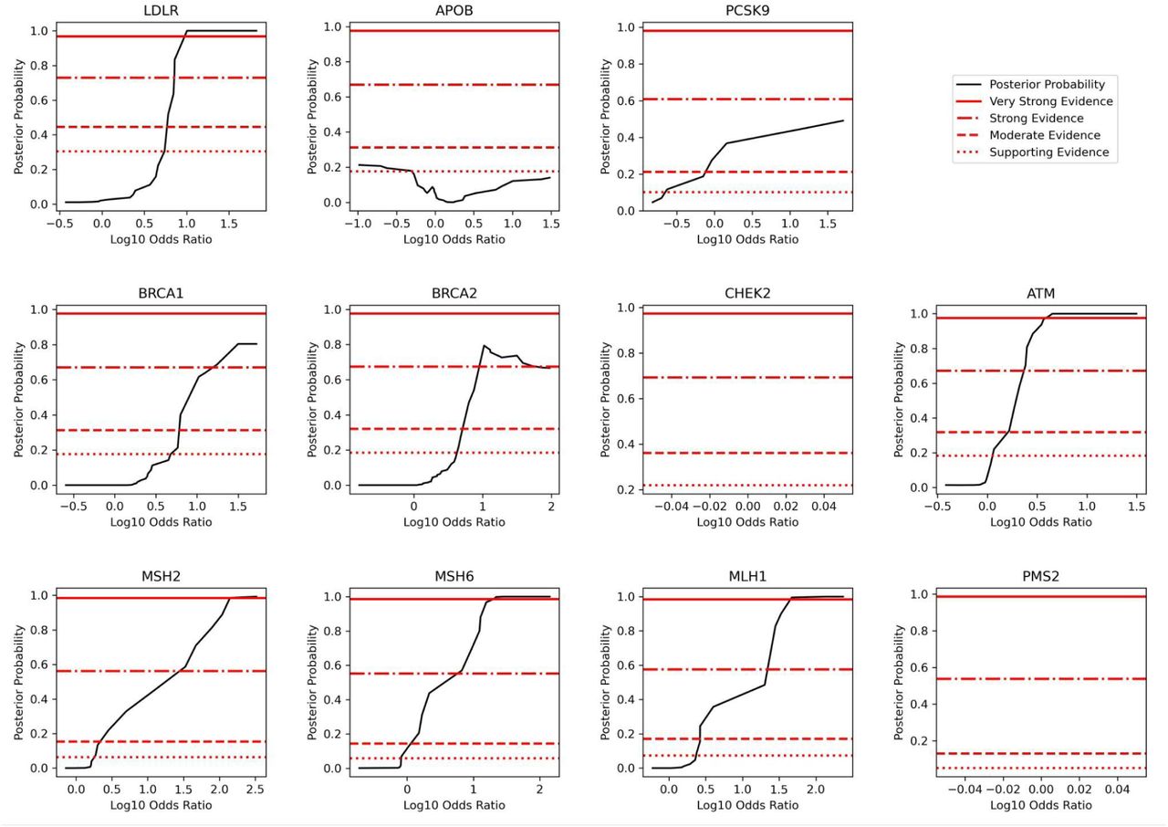
Using a version of the local posterior-probability based approach introduced in Pejaver et al., we calibrate population-based odds ratios and define evidence thresholds at the phenotype and gene levels. Notably, we use population-based priors that vary by phenotype and gene as described in Methods. Population-based odds ratios reach supporting and moderate evidence in all phenotypes (FH, HBOC, CRC), while in HBOC they reach strong evidence and in CRC they reach very strong evidence (Figure 2A). Evidence thresholds at the phenotype level are presented in Table 2A. At the gene level, odds ratios reached strong or very strong evidence in all genes except APOB (moderate evidence) and CHEK2 and PMS2, where calibration was not possible due to a lack of benign variants (Figure 2B, Supplementary Figure 3). Evidence thresholds at the gene level are presented in Table 2B, and bootstrapped results and confidence intervals are presented in Supplementary Figure 4. For consistency with previous approaches that calibrate on all available data, we also calibrate population-based odds ratios in aggregate across all 11 genes that are a part of our analysis, and find that odds ratios reach strong evidence (Supplementary Figure 5B). Aggregate evidence thresholds are presented in Supplementary Table 4.

[A] Posterior probability curves for variants in FH genes, HBOC genes, and CRC genes with 3 standard deviation gaussian smoothing. Note that the threshold levels used (supporting, moderate, strong, very strong) vary by plot since we estimate priors at the gene level and use a weighted average of gene priors to calculate phenotype-level priors, as described in Methods. Odds ratios reach a maximum of moderate evidence in FH genes, a maximum of strong evidence in HBOC genes, and a maximum of very strong evidence in CRC genes. [B] Posterior probability curves for variants in LDLR, APOB, and PCSK9 with 3 standard deviation gaussian smoothing. Horizontal lines correspond to evidence levels as described earlier. Odds ratios reach a maximum of strong evidence in BRCA1 and MSH2, and a maximum of very strong evidence in LDLR.
We calculated odds ratio intervals that correspond to different ACMG/AMP evidence strength levels in FH genes, HBOC genes, and CRC genes. A dash means that the specified level of evidence was either not reached or that insufficient data was available to calculate the range. Odds ratios reach strong or very strong evidence for all phenotypes except FH, where a maximum of moderate evidence was reached.
We calculated odds ratio intervals that correspond to ACMG/AMP evidence strength levels in all genes studied. A dash means that the specified level of evidence was either not reached or that insufficient data was available to calculate the range. Odds ratios reached strong or very strong evidence in all genes except APOB, CHEK2, and PMS2.
Comparing outcomes for participants with high odds ratio VUS versus pathogenic variants
We sought to identify potential differences in outcomes for participants with high odds ratio VUS and variants absent from ClinVar (VUS/absent) and high odds ratio P/LP variants, using survival analysis. Figure 3 shows comparisons in three key genes (LDLR, BRCA1, and MSH2) at various definitions of a high odds ratio threshold (5, 10, 15, and the optimal threshold described previously). Surprisingly, we found that outcomes for participants with VUS are not significantly different compared to those with P/LP variants at many thresholds (Figure 3). Notably, MSH2 VUS need to meet a much higher OR threshold compared to LDLR and BRCA1 to have outcomes not significantly different from participants with P/LP variants, highlighting differences in how population evidence might be evaluated at the gene level.

[A] Survival analysis of participants with no variants, P/LP variants with odds ratios ≥ 5, and VUS/absent variants with odds ratio ≥ 5 in (from left to right) LDLR, BRCA1, and MSH2. Survival curves were generated using a Kaplan-Meier estimator, and shaded regions represent 95% confidence intervals. “At risk” counts describe the number of participants considered in each of the three groups at different ages. Logrank p-values between P/LP and VUS survival curves are noted in each plot. [B] Survival analyses of participants with variants with odds ratio ≥ 10. [C] Survival analyses of participants with variants with odds ratio ≥ 15. [D] Survival analyses of participants with variants with odds ratio ≥ ‘optimal threshold’. Note that optimal thresholds refer to the thresholds described in Supplementary Table 3.
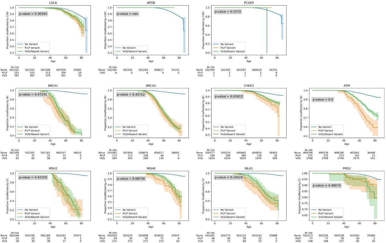
Among all genes, for variants with a population-based odds ratio ≥ 5 and the lower 95% confidence bound ≥ 1 (the ACMG/AMP recommended threshold for the application of PS4 evidence), outcomes among participants with VUS and variants absent from ClinVar were not significantly different from those with P/LP variants except in CRC genes MSH2 (logrank p = 4.7x10⁻¹⁴), MSH6 (logrank p = 0.03), and MLH1 (logrank p = 1.4x10⁻⁸), as well as BRCA2 (logrank p = 0.02) (Supplementary Figure 6). This indicates that PS4 evidence from population cohort data based on current guidelines – in aggregate – may be as strong as P/LP annotations in some of the genes we evaluated.
We next analyzed outcomes in all genes using the optimal odds ratio thresholds previously described (Supplementary Table 3), and find that there is no significant difference in outcomes between participants that have VUS/absent and P/LP variants with an odds ratio ≥ the optimal threshold in all genes except CHEK2 (p = 0.04), ATM (logrank p = 1.2x10⁻⁶) and APOB (no participants have P/LP variants with OR ≥ optimal threshold) (Supplementary Figure 7). Within CRC genes broadly, as with MSH2, a higher odds ratio threshold was needed in order for participants with VUS to have outcomes not significantly different from participants with P/LP variants. Specifically, we find that VUS in genes with lower effect sizes require higher OR thresholds.
Correlation between population evidence and computational and functional evidence
We analyzed the correlation between population-based odds ratios (PS4/population evidence) and REVEL scores (PP3/BP4/computational evidence) as well as functional scores (PS3/BS3/functional evidence) in 3 genes where these data sources were both available (LDLR, BRCA1, MSH2). Interestingly, we find that odds ratios are moderately correlated with REVEL scores in LDLR, but not in BRCA1 and MSH2 (Figure 4A), and that odds ratios are moderately correlated with functional scores in LDLR and BRCA1, but not in MSH2 (Figure 4B).

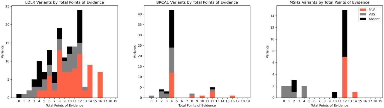
[A] Spearman correlation between log10 odds ratios and REVEL computational predictions of variant pathogenicity. [B] Spearman correlation between log10 odds ratios and functional estimates of variant impact from experimental assays. Odds ratios (population evidence) in LDLR are most concordant with computational, functional, and contextual evidence compared to BRCA1 and MSH2, where these sources were either less available or less concordant. [C] For variants with population evidence of pathogenicity, we recorded the number of variants with different forms of evidence (computational, functional, contextual).
We then sought to identify how many VUS and variants absent from ClinVar in these genes might have sufficient evidence to be classified as P/LP, making use of population, computational, and functional evidence criteria, as well as contextual evidence from previously classified pathogenic variants, which has been shown to be potentially underused.11 We evaluate each of these forms of evidence for variants where we have identified population evidence of pathogenicity, as described in the Methods. The number of variants with different forms of evidence in each of LDLR, BRCA1, and MSH2 is shown visually in Figure 4C. We combine these forms of evidence using the Bayesian framework based point system, noting that a comprehensive evaluation of all available forms of evidence would be required for a diagnostic variant interpretation. Overall, 60 VUS and variants absent from ClinVar (many, 80.0%, of which are in LDLR) affecting 245 participants can be presumptively classified as P/LP (points ≥ 6) across LDLR, BRCA1, and MSH2 (Supplementary Figure 8). More broadly, we find 563 VUS and variants absent from ClinVar with strong or very strong population evidence across all the genes we analyzed which affect 2,456 participants, highlighting the clinical value of population-based odds ratios.
Discussion
Our results demonstrate that population cohort data at scale can be used to directly estimate variant impacts at the nucleotide level. This can provide valuable information for variant assessment across a range of clinically actionable phenotypes. We found that UK Biobank population-based odds ratios reached ‘strong’ or ‘very strong’ evidence in 8 of the 11 genes we analyzed when applying the Bayesian adaptation of the ACMG/AMP framework.12 Collectively, many individuals harbor rare VUS in an actionable disease gene, and this framework can provide information to expedite the interpretation of these variants.
Calibration of evidence at the phenotype and gene level
We calibrated population evidence at the phenotype and gene level and calculated odds ratio thresholds which can be considered supporting, moderate, or strong evidence of pathogenicity. This approach extends prior calibration methods that use a single set of thresholds across all genes. Our approach involved calculating prior probabilities and local likelihood ratios for each gene and set of genes related to each phenotype. Given the wide variability we observed in evidence thresholds and the prevalence of pathogenic variants among different genes and genes related to each phenotype, this approach may be valuable in future calibration efforts when sufficient data is available.
Alternative approaches considered for calibration
Our calibration strategy followed a localized estimation approach introduced in Pejaver et al. with some minor changes described in Methods. We primarily contended between this localized approach and a global approach which involves calculating likelihood ratios using all available variants. As has been described previously, the primary disadvantage of a global approach is that only a single global threshold is considered, and any odds ratio value greater than that threshold would be considered to have the same strength of evidence, though this may not always be the case.13 Due to this challenge, we used a localized estimation approach, though we note that this also has limitations. Specifically, a local approach requires a large amount of data and may suffer from imprecision when the interval around a score used to calculate lr+ has to be very wide in order to include a sufficient number of variants for estimation. While the approach in Pejaver et al. maintained intervals wide enough such that 100 pathogenic or benign variants are always included. This approach was not always feasible with population data at the gene level given the low numbers of pathogenic or benign variants in some genes. Instead, we maintained intervals wide enough such that a variable number of pathogenic or benign variants are always included: this number was set to 20% of the total number of pathogenic or benign variants in a gene, as we found this to work particularly well, although alternative approaches may use a different proportion or a constant number.
Estimating the prevalence of pathogenic variants, or the prior probability, can be substantially different depending on the context. For example, Tavtigian et al. assumed 10% given the context of identifying a pathogenic variant among a set of candidate variants from clinical genetic testing, and Pejaver et al. estimated a lower number, 4.41%, empirically using gnomAD as a reference set. We contended between two methods to calculate the prevalence of pathogenic variants in a given gene: one using population data from the UK Biobank and the other using clinical diagnostic data from ClinVar, as described in Methods. We used population-based priors due to their concordance with our approach, though we also calculated priors based on clinical data (using non-pathogenic UK Biobank variants as controls) and found them to be generally lower than those based on population data. We note that other approaches based on clinical diagnostic data may make use of other control datasets such as gnomAD for this purpose, and that there are alternative ways to calculate prior probabilities outside of these two methods (e.g., using functional assay data).
Approaches to automating components of variant interpretation
Methods to automatically generate structured sources of diagnostic evidence can expedite variant assessment and prioritize the most promising variants for re-assessment. Notably, when combining four forms of evidence which we automatically generated (population, computational, functional, contextual), we found that 72.2% of VUS in LDLR with strong or very strong population evidence also have sufficient complementary evidence to be potentially classified as pathogenic, and that these VUS with sufficient evidence represent 12.4% of all rare VUS in LDLR seen in participants. Broadly, among participants with a rare variant in the genes we analyzed that reached strong or very strong evidence, 4.3% (N = 2,456) have a VUS or variant absent from ClinVar with strong population evidence that could be informative about increased risk of a related disorder. As functional assay data for additional genes are developed, and computational scores evolve, combining these automatable sources of evidence can help dramatically scale variant interpretation.
Limitations and future directions
In populations other than those most highly represented in the UK Biobank, there are an insufficient number of participants with rare missense variants to make robust estimates of risk. Therefore, we note that our estimates may not be generalizable to those other populations or those not ascertained during adulthood, and future work may estimate population-specific variant effects. Additionally, while our analysis focuses on a subset of actionable genes that are some of the most commonly screened in diagnostic settings, future work may analyze a broader set of genes. Given small variant counts at the gene level, we caution that gene-level calibration may be data-constrained, and that statistical estimates will become more powerful as biobank sizes grow. We provide higher confidence calibration thresholds in our fully aggregated calibration across all 11 genes we analyzed (Supplementary Table 4).
To remain consistent with ACMG/AMP guidelines and commonly used standards developed by variant curation expert panels (VCEPs), we use an odds ratio to represent enrichment of disease at the population level for individual variants. Future work may evaluate other representations of population evidence (e.g., using other statistical measures or models) to achieve better performance. We note that odds ratio estimates can be confounded by low variant allele counts or population structure. Separately, because we have focused on rare variants in genes where coding variants are known to have a substantial effect, we presume that these variants are likely to be truly causal. In rare cases, it is possible for a variant we analyzed to be tagged by a more common coding variant with functional effect, though this is unlikely to impact our calibration efforts which were aggregated at the gene level.
Conclusion
In summary, this analysis presents a comprehensive approach to assess the impact of germline variants using endophenotypic and disease risk data from a national biobank. For the set of genes we analyzed, we calculated variant-level odds ratios and calibrated strengths of evidence, then used these to identify VUS which can potentially be re-classified as pathogenic. By highlighting the utility of biobank data and calibrating it, we hope that this form of population evidence can be adopted to inform variant interpretation broadly.
STAR ★ Methods
Key resources table
Resource availability
Lead contact
Requests should be directed to and will be fulfilled by the lead contact, Christopher A. Cassa (ccassa{at}bwh.harvard.edu).
Materials availability
This study did not generate new unique reagents.
Experimental model and subject details
No experimental models or novel subjects were utilized or collected as part of this publication.
Method details
Study participants
The UK Biobank is a prospective cohort of over 500,000 individuals recruited between 2006 and 2010, ages 40-69.26 Among the 469,803 participants with whole exome sequencing data, we evaluated rare non-synonymous variants present in genes related to the following phenotypes: familial hypercholesterolemia (FH; APOB, LDLR, PCSK9), hereditary breast and ovarian cancer syndrome (HBOC; BRCA1, BRCA2, CHEK2, ATM), and Lynch syndrome (CRC; MLH1, MSH2, MSH6, PMS2). We excluded participants who either had missing phenotypic data, who had more than one rare (AF <= 0.1%) non-synonymous variant across the set of genes related to each phenotype, or who had a rare non-synonymous homozygous variant.
Variant inclusion, quality control, and annotations from exome sequencing data
Sequencing and transcripts
Whole exome sequencing (WES) was performed for UK Biobank participants, as previously detailed.9 Analysis was conducted on the UK Biobank DNAnexus Research Analysis Platform (https://ukbiobank.dnanexus.com). We extracted gene-level VCF files from WES pVCFs and normalized to flatten multi-allelic sites using bcftools (v1.15.1) and the Swiss Army Knife application (v4.9.1).27 Exon coordinates were identified from MANE transcripts, with an additional 5 nucleotides retained upstream and downstream of each coding region to capture splice-site variants.
Quality control
Variants in low complexity regions, segmental duplications, or other regions known to be challenging for next generation sequencing alignment or calling were removed from analysis (NIST GITB difficult regions),28 as were variants with an alternate allele frequency greater than 0.1% in the UK Biobank cohort.9 Further filtering removed variants in which more than 10% of samples were missing genotype calls. To mitigate differences in sequencing coverage between individuals who were sampled at different phases of the UK Biobank project, variants were only retained in the final set if at least 90% of their called genotypes had a read depth of at least 10.
Annotations
The canonical functional consequence of each variant was calculated using Variant Effect Predictor (v108).19 Non-coding variants outside of essential splice sites were not considered in the analysis, and non-synonymous coding variants were included with any of the following canonical consequences: “splice_acceptor_variant”, “splice_donor_variant”, “stop_gained”, “frameshift_variant”, “stop_lost”, “start_lost”, “missense_variant”, “inframe_insertion”, “inframe_deletion”. REVEL scores were aggregated from all available transcripts and annotated if available in at least one transcript.
Clinical endpoints and endophenotypes
Primary clinical endpoints were specific to each condition: adjusted LDL-C levels for FH, female breast or ovarian cancer cases for HBOC, and colorectal cancer cases for CRC. Case definitions were defined in the UK Biobank using a combination of self-reported data confirmed by trained healthcare professionals, hospitalization records, and national procedural, cancer, and death registries. Age at event was estimated based on listed date of event and birth date when not directly provided, and cases with unavailable event data were excluded. Estimated untreated (adjusted) LDL-C levels were derived using adjustments for lipid-lowering therapies, as applied previously.29 Adjusted LDL-C levels were subsequently used to calculate odds ratios in FH genes, with 190 mg/dL as the threshold value. For HBOC and CRC, breast or ovarian cancer and colorectal cancer cases were used to calculate odds ratios, respectively.
Calculating variant-level odds ratios from population cohort data
Variant-level odds ratios were calculated using the aforementioned endophenotype and disorder case data, where for a non-synonymous variant 𝑣 the “population-based odds ratio”
 Haldane-Anscombe correction (adding 0.5 to all cells 𝑎, 𝑏, 𝑐, 𝑑 in the contingency table) was applied to allow for the calculation of odds ratios when no false positives existed, while also reducing the bias of the estimator. Variants for which 𝑎 was 0 and the corrected odds ratio was ≥ 1 were not included in analyses.
ClinVar clinical assertions from diagnostic laboratories
ClinVar summary assessments were extracted from the tab delimited ClinVar variant summary file released on 04/06/2023.30 We grouped ‘pathogenic’, ‘likely pathogenic’, and ‘pathogenic/likely pathogenic’ classifications as ‘P/LP’ collectively, and grouped ‘benign’, ‘likely benign’, and ‘benign/likely benign’ classifications as B/LB. Importantly, we used the term VUS inclusively to capture all variants with an inconclusive classification: including “uncertain significance,” “conflicting interpretations of pathogenicity,” and “not provided”.
Calibrating population evidence of pathogenicity (PS4)
Estimating the prevalence of pathogenic variants
We considered two methods for estimating the prevalence of pathogenic variants, or the prior probability of pathogenicity: 1) using population data from the UK Biobank and 2) using clinical data from ClinVar. In the first approach, we estimate the prior probability of pathogenicity in a gene 𝑔 as
 Then, priors at the phenotype level can be calculated as the weighted average
 A similar weighted average can be used to aggregate phenotype-level priors into an overall prior for all phenotypes considered. Often, in previous studies, a single overall prior has been calculated for calibration across all genes in a dataset; however, we contend that there is a benefit to stratifying at the phenotype and gene level given how widely priors can differ at these levels.12,13 We report prior probabilities of pathogenicity generated using population data in Supplementary Table 1A. The prior for variants in Lynch syndrome genes was particularly low (2.5%), while the prior for variants in LDLR was particularly high (19.3%). Notably, the overall aggregated prior of 8.0% is similar to the 10% prior assumed in Tavtigian et al.12
In the second approach, we estimate the prior probability of pathogenicity in a gene 𝑔 as
 Weighted averages can be calculated for phenotype-level and overall prevalence values of pathogenic variants, as described earlier. We report priors generated using clinical data in Supplementary Table 1B. Compared to priors based on population data, these priors were generally higher in Lynch syndrome genes and lower in all other genes with the exception of LDLR which was slightly higher at 20.1%. Notably, the overall aggregated prior of 5.4% is similar to the 4.41% calculated in Pejaver et al.13
We caution that both of our methods to estimate pathogenic variant prevalence may underestimate true values. When using population case data from the UK Biobank, there are participants that are yet to develop a phenotype, and when considering the proportion of ClinVar P/LP variants among nonsynonymous variants in the UK Biobank, there are a large number of nonsynonymous variants observed in the UK Biobank that are not represented in ClinVar. For subsequent analysis, we use population-based priors, as they align well with our existing approach for calculating odds ratios.
Statistical framework
The ACMG/AMP variant interpretation guidelines describe multiple levels of strength in favor of variant pathogenicity: supporting, moderate, strong, and very strong.6 These strength levels have been mapped to positive likelihood ratios (LR+) to quantify variant impact.12 To calibrate the strength of population evidence (which we model as continuous odds ratios) at the gene level, we use a sliding window method similar to that introduced in Pejaver et al. for the calibration of computational scores.13 For every population odds ratio 𝑝, we calculate a local likelihood ratio (lr+) using pathogenic and benign variants with odds ratios in the interval [𝑝 − 𝑧, 𝑝 + 𝑧] for the lowest value of z such that {𝑣 | 𝑂𝑅(𝑣) ∈ [𝑝 − 𝑧, 𝑝 + 𝑧]} contains at least 20% of all pathogenic and benign variants in a given gene excluding those for which odds ratios could not be calculated. The local likelihood ratio calculation is then
 Given this and the prior probability of pathogenicity 𝑎, we can calculate the posterior probability of pathogenicity 𝑏 for a variant by rearranging the following equation:
 Next, to map supporting, moderate, strong, and very strong evidence thresholds to posterior probability thresholds for each gene and phenotype, we calculate suitable values for the odds of pathogenicity for very strong evidence (𝑂PVst). This value was determined using the supplementary table from Tavtigian et al. so that the ACMG/AMP combining rules are generally satisfied and the posterior probability reaches the values of 0.9 and 0.99 for likely pathogenic and pathogenic classifications, respectively. The map from prior probabilities to O values is reported in Supplementary Table 2. We then used the 𝑂PVst values for each gene and phenotype as the lr+ variable in the equation above to calculate the very strong posterior probability threshold for that gene/phenotype. For strong, moderate, and supporting evidence of pathogenicity, this process was repeated but using
  , respectively, based on the assumption that evidence levels scale by powers of 2.
Finally, to identify intervals of population-based odds ratios that correspond to varying levels of evidence, we identify the minimum odds ratio at which the posterior probability threshold for an evidence level is crossed, then use linear approximation to estimate the odds ratio at which the exact threshold would be reached.
Survival analysis
Survival analyses including Kaplan-Meier curves and logrank tests were performed using the Python lifelines survival analysis package (v0.23.9).21
Conversion of evidence to the point system
To identify how many VUS and variants absent from ClinVar with population evidence might have sufficient evidence to be classified as P/LP, we considered multiple evidence sources and converted them to the semi-quantitative point system adaptation of the ACMG/AMP sequence variant interpretation framework.31 We interpreted variants with ORs greater than the strong/very strong thresholds presented in Table 2B as having PS4 evidence (+4 points on the point scale). REVEL scores were converted to evidence bands (PP3/BP4) using thresholds calculated in Pejaver et al.,13 and functional scores were translated to PS3 (+4 points) or BS3 (-4 points) based on author recommended thresholds, with the exception of LDLR, where a threshold wasn’t provided and which we estimated by analyzing global LR+ with ClinVar as a truth set.16–18 Finally, contextual evidence from previously classified pathogenic variants was applied in the following manner: PVS1 (+8 points) for LOF variants annotated as high-confidence by LOFTEE,32 PS1 (+4 points) when a variant has a colocated P/LP variant encoding the same substitution and -4 points when a variant has a colocated B/LB variant encoding the same substitution (note that the benign equivalent is not an established ACMG/AMP criterion), and PM5 (+2 points) when a variant has a colocated P/LP variant encoding a different substitution and -2 points when a variant has a colocated B/LB variant encoding a different substitution (note that the benign equivalent is not an established ACMG/AMP criterion).
Data availability
Population-based variant odds ratios and the underlying case-control data used in their calculation are available at https://doi.org/10.6084/m9.figshare.c.7169472.v1 for all genes studied.

The distribution of log10 odds ratios by ClinVar status in all genes studied. Odds ratios significantly separate pathogenic and benign variants in all genes except APOB (p = 0.17), PCSK9 (p = 0.07), CHEK2 (no benign variants), and PMS2 (no benign variants).

ROC curves for classification of ClinVar variants using population odds ratios for all genes studied. AUC was between 0.90 and 1.00 in all genes except APOB (0.33), CHEK2 (no benign variants), and PMS2 (no benign variants).

Posterior probability curves for variants in all genes studied with 3 standard deviation gaussian smoothing. Note that the threshold levels used (supporting, moderate, strong, very strong) vary by plot since we estimate priors at the gene level, as described in Methods. Odds ratios reached strong or very strong evidence in all genes except APOB (moderate evidence), as well as CHEK2 and PMS2, where calibration was not possible due to a lack of benign examples.

Estimated posterior probability curves for variants in all genes studied with 3 standard deviation gaussian smoothing. Posterior probability estimates and confidence bounds were derived via 10,000 bootstrapping iterations, where the estimate, lower bound, and upper bound were the mean, 5th percentile, and 95th percentile of the bootstrapped distribution, respectively.

[A] Odds ratios significantly separate pathogenic and benign variants in aggregate (p = 2.1x10-73). [B] Posterior probability curve across all genes in aggregate with 3 standard deviation gaussian smoothing. Odds ratios reach strong evidence in aggregate using the prior of 8.0% (OPVst = 480) shown in Supplementary Table 1A. [C] ROC curve for classification of ClinVar variants using population odds ratios in aggregate (AUC = 0.94).

Survival analysis of participants with no variants, P/LP variants with odds ratio ≥ 5, and VUS/absent variants with odds ratio ≥ 5 in all genes studied. Survival curves were generated using a Kaplan-Meier estimator, and shaded regions represent 95% confidence intervals. “At risk” counts describe the number of participants considered in each of the three groups at different ages. Logrank p-values between P/LP and VUS survival curves were not significantly different in all but 4 genes: MSH2 (logrank p = 4.7x10⁻¹⁴), MSH6 (logrank p = 0.03), MLH1 (logrank p = 1.4x10⁻⁸), and BRCA2 (logrank p = 0.02).

Survival analysis of participants with no variants, P/LP variants with odds ratio ≥ optimal threshold, and VUS/absent variants with odds ratio ≥ ‘optimal threshold’ in all genes studied. Survival curves were generated using a Kaplan-Meier estimator, and shaded regions represent 95% confidence intervals. “At risk” counts describe the number of participants considered in each of the three groups at different ages. Logrank p-values between P/LP and VUS survival curves were not significantly different in all genes except CHEK2 (p = 0.04), ATM (logrank p = 1.2x10⁻⁶) and APOB (no participants have P/LP variants with OR ≥ optimal threshold).

When applying the ACMG guidelines, we calculated the number of points of evidence from population, computational, functional, and contextual data sources for variants in LDLR, BRCA1, and MSH2 for variants that have ‘strong’ or ‘very strong’ population evidence, separated by ClinVar status. Notably, 60 VUS and variants absent from ClinVar reach ≥ 6 points, most of which are concentrated in LDLR.
Prior probabilities of pathogenicity estimated as 𝑃(𝑓|𝑣) as described in Methods for all genes studied. Prior probabilities at the phenotype level were estimated by taking a weighted average of priors in associated genes, and an overall prior probability was estimated by taking a weighted average of all phenotype priors. Notably, the overall prior of 8.0% is not very different from the 10% assumed in Tavtigian et al., and, we find that prior probabilities can vary greatly at the phenotype and gene level.
Prior probabilities of pathogenicity are estimated using the proportion of ClinVar P/LP variants for all genes studied. Prior probabilities at the phenotype level were estimated by taking a weighted average of priors in associated genes, and an overall prior probability was estimated by taking a weighted average of all phenotype priors. Notably, the overall prior of 5.4% is not very different from the 4.41% calculated in Pejaver et al., and we again find that priors can vary greatly at the phenotype and gene level.
We map between prior probabilities of pathogenicity estimated using population data and the value of OPVst used for calibration, at the phenotype level (top) and gene level (bottom).
Odds ratio thresholds at which specificity and sensitivity are maximized (using the Youden Index or most upper left point on each ROC curve, which can also be interpreted as the point at which global LR+ is maximized), at the phenotype level (top) and gene level (bottom).
We calculated odds ratio intervals that correspond to ACMG/AMP evidence strength levels in aggregate across all genes studied using the prior of 8.0% (OPVst = 480) shown in Supplementary Table 1A. A dash means that the specified level of evidence was either not reached or that insufficient data was available to calculate the range. Odds ratios reached strong evidence overall.
Acknowledgments
We are indebted to the UK Biobank and its participants who provided biological samples and data for this study, performed under UK Biobank application 41250 and Mass General Brigham IRB protocol 2020P002093. We gratefully acknowledge funding from NIH R01HG010372 (V.B., T.Y., L.B., C.A.C.), NIH R01HG013350 (V.P.) and R56HG012681 (T.Y., C.C.).
Footnotes
Declaration of Interests: The authors declare no competing interests.
References


