
Abstract
Malaria is a life-threatening disease which has caused enormous public health challenge. A mathematical model describing the dynamics of malaria between the human and vector population is formulated to understand the important parameters in the transmission and develop effective prevention and control strategies. We analysed the model and found that the model has a disease-free equilibrium (DFE) which is locally and globally asymptotically stable if the effective reproduction number can be brought below unity. Our model shows that the infectivity of mildly infected children and adults amplifies the disease burden in a population. It was shown that the model does not undergo the phenomenon of backward bifurcation so long as the recovered children and adults do not lose their acquired immunity and if the infection of mildly infected adult is not high enough to infect susceptible mosquitoes. However, control strategies involving mosquito reduction through high rate of application of insecticide will serve as an effective malaria control strategy. It is further shown that whenever the effective reproduction number is greater than unity the model has a unique endemic equilibrium which is globally stable for the case when there is loss of acquired immunity in children and adults. Numerical simulations show that the presence of all the control strategies is more effective in preventing mild malaria cases in adult and children as compared to severe malaria cases in adult and children.
1 Introduction
Malaria poses a substantial public health problem with about 228 million cases worldwide and 405,000 deaths globally [1]. Majority of this malaria burden up to 93% occur in Africa of which 85% is within the sub-Saharan Africa, of which Nigeria bears 25% of this burden. Hence, the country with the highest malaria burden [1]. Children under 5 years of age are the most affected and an increasing re-emergence of some severe clinical manifestation in adults is likely [1–3]. Malaria is a life-threatening disease that is transmitted through the bites of infected female anopheles mosquito (vector). After entering a human, the parasites transform through a complicated life-cycle in the liver and bloodstream. A stage in the life cycle developed into gametocytes, which spreads through a susceptible mosquito that bites the infectious human [3]. After approximately 10 to 15 days the mosquito takes her next blood meal and can infect a new person. After a human gets bitten, the symptoms appear in about 9-14 days. Clinical symptoms such as fever, pain, chills and sweats may develop a few days after infected mosquito bites. The infection can lead to serious complications affecting the brain, lungs, kidneys and other organs [3–5]. Since malaria increases morbidity and mortality, it continues to inflict major public health and socioeconomic burdens in developing countries. Malaria control even in countries with relatively low malaria endemicity proves to be a significant challenge. The complexity of the disease control process, the cost of the control programme and resistance of the parasite to anti-malarial drugs, and vectors to insecticides, are some of the challenges [3, 4, 6]. The rate of acquisition of immunity to severe malaria depends on age distribution of humans and the level of exposure to infections [7, 8]. Recently, the international community has increased its focus on eradicating malaria burden worldwide [1].
The battle towards the eradication and or control of malaria would have to take a collaborative approach to be achieved. Partly involving the role of mathematicians and their modelling approach in studying the dynamics of malaria, giving an insight into the interaction between the host and vector population and how to control its transmission. This is a collaborative work aimed at constructing a vector-borne compartmental model in a heterogeneous population incorporating mosquito reduction strategy, personal protection strategy, vaccination as control strategies and immune compartments in both children and adult population. This work considers all of these control strategies, which were not completely captured in previous report [8–10].
2 Model Formulation
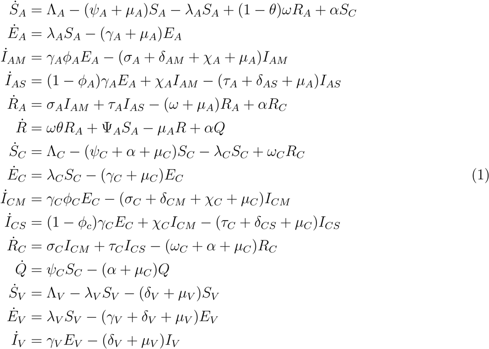
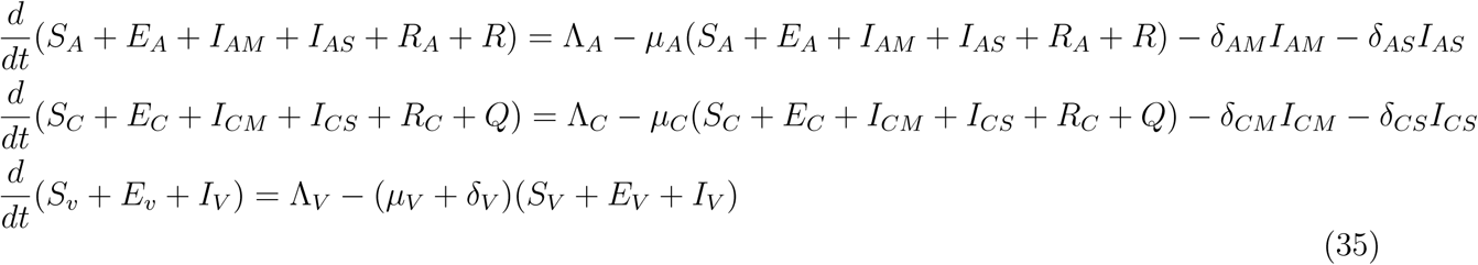
A mathematical model for endemic malaria is formulated in a heterogeneous population with two human populations consisting of adults and children. The vector (mosquito) population is considered in this work where NA(t), NC(t) and NV (t) denote the total number of adults, children and vectors at time t, respectively. As specified in (Table 2.1), the total population of human and vectors is divided into the following mutually exclusive epidemiological classes, namely, susceptible adults (SA(t)), adults with asymptomatic malaria (EA(t)), adults with malaria at mild stage (IAM (t)), adults with severe malaria (IAS(t)), adults treated of malaria (RA(t)), immune adults (R(t)), susceptible children (SC(t)), children with asymptomatic malaria (EC(t)), children with mild malaria (ICM (t)),children with severe malaria (ICS(t)),children treated of malaria (RC(t)), immune children (Q(t)), susceptible vectors (SV (t)), vectors with parasite at latent stage(EV (t)), vectors with parasite(IV (t)), Hence, we have that in,

Flow diagram of malaria model
Susceptible adults contact malaria with disease force of infection rate
 Susceptible children contact malaria at a rate
 Susceptible vectors acquire the gametocytes from infected humans at a rate
 Susceptible children and adults are recruited at rates ΛC, ΛA while the susceptible mosquitoes are recruited at a rate ΛV (Table 2.1). Also, susceptible adults and children are vaccinated at rates ψA, ψC respectively. We assume that fraction ϕA, ϕC of adults and children with asymptomatic malaria progress to the mild stage of infection (at rates γA, γC respectively) while remaining fraction 1 − ϕA, 1− ϕc of adults and children progress to the severe stage of infection (at rates γA, γC).
Let βA, βC, βV represent transmission probability per contact for adults, children and susceptible mosquitoes. Infected adults at mild and severe stages of infection progress to class of recovered adults at rates σA, τA respectively, while infected children at mild and severe stages of infection progress to class or recovered children at rates, σC, τC respectively.
The parameters δAM, δAS, δCM, δCS, represent the disease induced death rates for adults and children at mild and severe stage respectively. δV represent the death rate of mosquitoes from insecticide. The parameters θ represent the fraction of recovered adults who develop immunity after recovery while 1 − θ represent the remaining fraction of recovered adults who become susceptible after treatment. bV is the mosquito biting rate while q is the rate of insecticide treated nets (ITN) compliance, ω represent the rate at which recovered adults revert to either the immune or susceptible adult class while ωC is the rate at which recovered children revert to susceptible children class. Vectors at latent stage become infectious at the rate γV. The parameters ηA, ηC represent the infectivity modification parameters in adults and children. η is a modification parameter that indicates that children exposure rate is different from that of adults. That is, children protected from mosquito bites are less likely to get malaria infections. We assume that the infection in the mild classes might not be high enough to infect susceptible mosquitoes or is at the same level as the infectious individual giving 0 ≤ ηC, ηA ≤ 1.
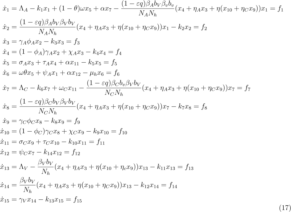
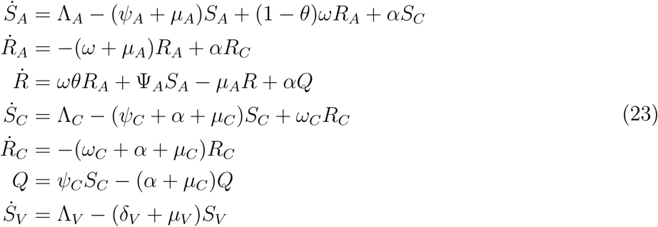
The model equations are given below
2.1 Basic Properties
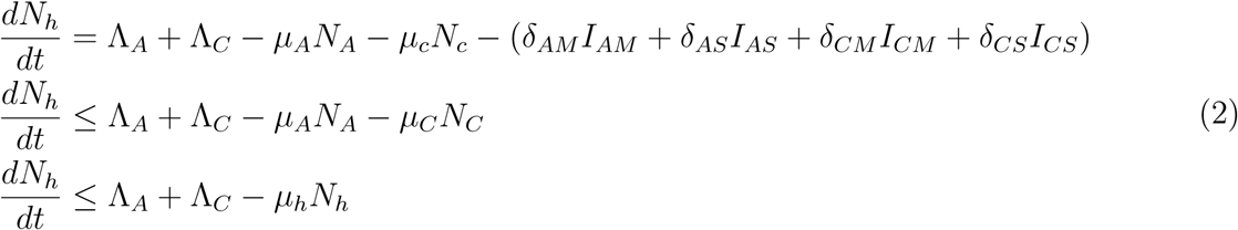
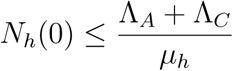
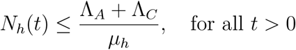
Since the model monitors both human and mosquito population during malaria epidemic, it is important to prove that all the state variables of the model are non-negative for all time (t) for the model (1) to be epidemiologically meaningful. That is, the solutions of the model (1) with positive initial data will remain positive for all time t > 0. Model (1) is basically divided into two regions, thus D = D1 × D2.
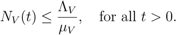
2.1.1 Boundedness
The region D = D1 × D2. of system (1) is positively invariant with non-negative initial conditions in 
Proof: The rate of change of the total human population is given as
Description of the variables and parameters of the Malaria model
Where μh = min {μA, μC}
A standard comparison theorem [11] can then be used to show that
 In particular, if
 then,
then,
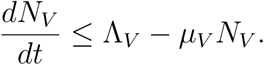
 The rate of change of the total vector population is given as
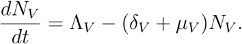 By standard comparison theorem,
 Solving gives
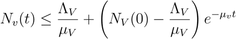 In particular, if
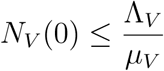 then,
then,
 Then either the solution enters D in finite time or NV (t) approaches
  as t → ∞. Thus, the region D = D1 × D2 is positively invariant so that no solution path leaves through any boundary of D. Thus the feasible solution of the human population is in the region
 and the feasible solution of the vector population is in the region
 Hence it is sufficient to consider the dynamics of the model (1) in the region. In this region, the model can be considered as being mathematically and epidemiologically well posed. Hence, the solution set of model (1) are contained in D.
2.2 Positivity of Solutions
We assumed that the initial conditions of the model are non-negative and we also showed that the solution of the model is also positive.
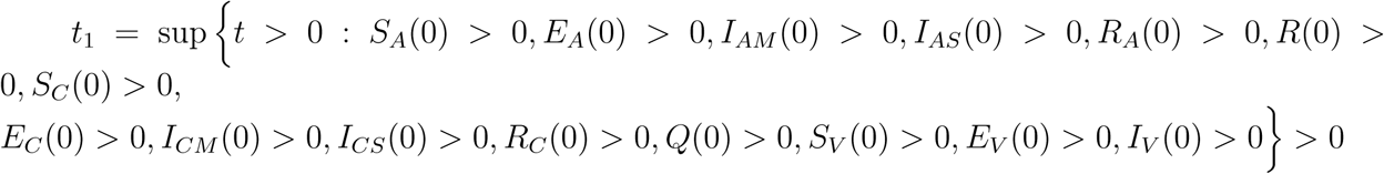
Let the initial data for the model be
SA(0) > 0, EA(0) > 0, IAM (0) > 0, IAS(0) > 0, RA(0) > 0, R(0) > 0, SC(0) > 0, EC(0) > 0, ICM (0) > 0, ICS(0) > 0, RC(0) > 0, Q(0) > 0, SV (0) > 0, EV (0) > 0, IV (0) > 0, then the solutions (SA, EA, IAM, IAS, RA, R, SC, EC, ICM, ICS, RC, Q, SV, EV, IV) of the model (1) with initial data will remain positive for all time t > 0.
Proof:
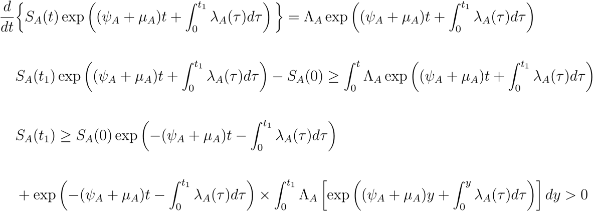
From the first equation in model (1)
 which implies
 Using integrating factor method, we have
 Similarly, it can be shown that all state variables of the model remain positive for all time t > 0 EA(t) > 0, IAM (t) > 0, IAS(t) > 0, RA(t) > 0, R(t) > 0, SC(t) > 0, EC(t) > 0, ICM (t) > 0, ICS(t) > 0, RC(t) > 0, Q(t) > 0, SV (t) > 0, EV (t) > 0, IV (t) > 0 for all time t > 0.
3 Analysis of the Model
3.1 Local stability of the disease-free equilibrium(DFE)
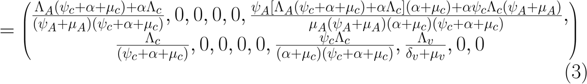
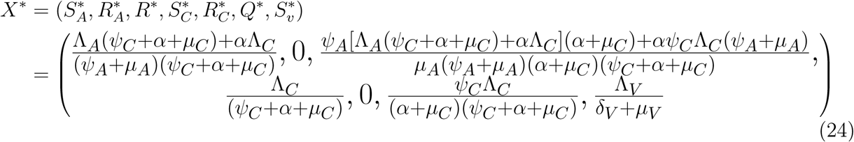
The disease-free equilibrium of the model (1) is given by

 Using the next generation operator method previously described [12],the local stability of ξ0 can be established, it follows that matrices, F and V for the new infection terms and the remaining transition terms are respectively given by
 and
and
 where,
 It follows that the effective reproduction number of model (1) denoted by ℛE is given by


 The result below follows from Theorem (2) in [12].
The DFE ξ0 of model (1) is locally asymptotically stable (LAS) if ℛE < 1, and unstable if ℛE > 1
The threshold quantity ℛE, is the average number of malaria cases generated by a typically infected individual introduced into a completely susceptible population. The expression ℛC is the number of secondary infections in children introduced by one infectious mosquito, while the expression ℛA is the number of secondary infections in adult introduced by one infectious mosquito. The biological significance of lemma 3 is that malaria can be adequately controlled in a community with children and adults if the quantity ℛE can be reduced to a value less than unity (ℛE < 1)
3.2 Analysis of the Control Reproduction Number
The threshold quantity, will be used to determine the effect of the control parameters ℛE on the eradication of malaria in the population. For the sake of mathematical tractability in the analysis of our malaria transmission model, we shall work with the square of the reproduction number since our conclusion will not be altered if the actual expression of the reproduction number is used [13, 14]. From (4), we have


 . It therefore follows that control programme that results in high treatment rates and ITN compliance (σA, τA, σc, τc, δv → ∞) can lead to effective malaria control if these result in the respective right-hand sides of (5a-5d) being less than unity. From (5e), a near total eradication of malaria is achievable. This implies that focusing on reducing mosquito population through high rate of application of insecticide will serve as an effective malaria control strategy. Thus, differentiating the square of the reproduction number,
  , given in (4) partially with respect to the parameters (σA, τA, σC, τC), further reveals the effect of these parameters on malaria control in the community. Thus,


3.3 Assessing the Impact of the Mild Classes
Differentiating the square of the reproduction number,  , given in (4) partially with respect to the parameters (ηA, ηc) [13, 15] gives

 This means that the square of the effective reproduction number,
  , is an increasing function of the parameters (ηA, ηc). Thus, the disease burden of malaria in the community will increase as the infectivity of mildly infected children and adults increases. However, taking the limit of 2 as (ηA, ηc 1) implies that the infectivity of mildly infected children and adults is the same as that of the severely infected adults and children. Thus,
 This implies that, as the infectivity of the mildly infected children and adults increases, the disease burden increases thereby increasing the number of malaria infected individuals in the community.
3.4 Existence of Endemic Equilibrium Point (EEP) of the Model
The model (1) has a unique endemic(positive) equilibrium for the special case when ω = ωC = α = 0 whenever ℛE > 1
See Appendix for the proof of Lemma 4.
3.5 Bifurcation Analysis of the Model
It is important to explore the existence of bifurcation as this will go a long way in determining the parameter that will hinder the possibility of eradicating malaria transmission if the reproduction number is less than one. The centre manifold theorem is used here to investigate possibility of the existence of backward bifurcation as described [14, 16, 17].
The transformed model (2) will undergo a backward bifurcation if the bifurcation coefficient a is positive
See Appendix for the proof of Lemma 5.
3.6 Global Asymptotic Stability of DFE
The DFE of the model (1) is globally asymptotically stable (GAS) in D whenever ℛE ≤ 1
See Appendix for the proof of Lemma 6.
3.7 Global Asymptotic Stability of EEP
The EEP of the model (1) is globally asymptotically stable (GAS) in D whenever ℛE > 1
See Appendix for the proof of Lemma 7.
4 Analysis of Control Strategies
To effectively study the behavioral pattern of malaria transmission, some important parameters of the model are explored here to quantify the effectiveness of malaria intervention strategies. We now carry out numerical analysis to investigate the relative importance of the parameters of our model in disease transmission and how best to tackle malaria outbreak and reduce malaria mortality. In particular, we target intervention strategies using parameters such as mosquito recruitment rate (ΛV), mosquito death rate (δV), mosquito biting rates (bV), rate of ITN compliance (q), vaccination rates (ψA, ψC) and treatment rates (σA, τA, σC, τC). Theoretical values are used to represent parameter values and initial conditions in our simulations since they are similar to comparable parameters for other mosquito-transmitted diseases [13, 14].
4.1 Mosquito-Reduction Strategy
The use of indoor residual spraying (IRS) and DDT reduce the average lifespan(δV)of mosquitoes and mosquito recruitment rate/birth rate (ΛV)respectively. The following three levels of mosquito-reduction strategies are considered for simulation [13, 15]
Description of parameter values
Low mosquito-reduction strategy
ΛV = 33334/day; δV = 0.25 /day
Moderate mosquito-reduction strategy
ΛV = 16667/day; δV = 0.5 /day
High mosquito-reduction strategy
ΛV = 8334/day; δV = 0.75 /day
Fig (1a) and (1c) indicate a decreasing pattern in both adult and children population with mild malaria while varying the recruitment rate of mosquitoes whereas Fig (1b) and (1d) show that adult and children population with severe malaria increase to a maximum value before they start decreasing gradually while varying mosquito recruitment rate.

Simulation of the Malaria model (1) for various control levels of the mosquito reduction strategy. (1a). New cases of adult population with mild malaria. (1b). New cases of adult population with severe malaria. (1c). New cases of children population with mild malaria. (1d) New cases of children population with severe malaria. The parameter values used are in Table2.1 with q = 0, ψA = 0, ψC = 0, δV = 0, σA = 0, σC = 0, τC = 0, τA = 0,
Fig (2a) and (2c) indicate a decreasing pattern in both adult and children population with mild malaria irrespective of the level of mosquitoes insecticide spray applied whereas Fig (2b) and (2d) show that high effectiveness mosquito reduction strategy lead to a considerable reduction in the number of severe malaria cases in adult and children population compared to the moderate-effectiveness level [13, 15].

Simulation of the Malaria model (1) for various control levels of the mosquito reduction strategy. (2a). New cases of adult population with mild malaria. (2b). New cases of adult population with severe malaria. (2c). New cases of children population with mild malaria. (2d) New cases of children population with severe malaria. The parameter values used are in Table 2.1 with q = 0, ψA = 0, ψC = 0, σA = 0, σC = 0, τC = 0, τA = 0,
4.2 Personal Protection Strategy
Personal protection involving the use of ITN (q)reduces the exposure rate of humans to mosquitoes which in turn reduces biting rates (bV) and the transmission of parasites between humans and (bV) mosquitoes. We consider the following three levels [13];
Low personal protection strategy
q = 0.133/day; bV = 0.75 /day
Moderate personal protection strategy
q = 0.265/day; bV = 0.50 /day
High personal protection strategy
q = 0.53/day; bV = 0.25 /day
In Fig (3a) and (3d),mild malaria cases in adult reduces faster within a shorter period as compared to mild malaria cases in children whereas Fig (3b) and (3c) show that with high personal protection strategy (use of insecticide treated nets) the number of severe malaria cases in adult and children population increase considerably to a level before decreasing gradually.

Simulation of the Malaria model (1) for various control levels of the mosquito reduction strategy. (3a). New cases of adult population with mild malaria. (3b). New cases of adult population with severe malaria. (3c). New cases of children population with mild malaria. (3d) New cases of children population with severe malaria. The parameter values used are in Table 2.1 with ψA = 0, ψC = 0, δV = 0, σA = 0, σC = 0, τC = 0, τA = 0,
In Fig (4a) and (4c), mild malaria cases in adult reduces faster within a shorter period as compared to mild malaria cases in children except when the biting rate is low in children population whereas Fig (4b) and (4d) show that when there is low personal protection strategy (high biting rate)the children population with severe malaria will increase more compared to the moderate-effectiveness level and high-effectiveness level.

Simulation of the Malaria model 1 for various control levels of the mosquito reduction strategy. (4a). New cases of adult population with mild malaria. (4b). New cases of adult population with severe malaria. (4c). New cases of children population with mild malaria. (4d) New cases of children population with severe malaria. The parameter values used are in Table2.1 with q = 0, ψA = 0, ψC = 0, δV = 0, σA = 0, σC = 0, τC = 0, τA = 0
4.3 Vaccination Strategy
Low vaccination strategy
ψA = 0.25/day; ψC = 0.25/day
Moderate vaccination strategy
ψA = 0.5/day; ψC = 0.5/day
High vaccination strategy
ψA = 0.75/day; ψC = 0.75/day
In Fig (5a) and (5b), susceptible adult and children population reduces faster due to vaccination whereas Fig (5c) and (5d) show that vaccination increases the immune adult and children population.

Simulation of the Malaria model (1) for various control levels of the mosquito reduction strategy. (5a). New cases of susceptible adult population. (5b). New cases of susceptible children population. (5c). New cases of immune adult population (5d) New cases of immune children population. The parameter values used are in Table 2.1 with q = 0, δV = 0, σA = 0, σC = 0, τC = 0, τA = 0
4.4 Combined Strategy
This strategy combines the mosquito reduction, personal protection and vaccination strategy under the following three control levels;
Low Combined Control
ΛV = 33334/day; δV = 0.25/day; q = 0.133/day; bV = 0.75/day; ψA = 0.25/day; ψC = 0.25/day
Moderate Combined Control
ΛV = 16667/day; δV = 0.5/day; q = 0.265/day; bV = 0.50/day; ψA = 0.5/day; ψC = 0.5/day
High Combined Control
ΛV = 8334/day; δV = 0.75/day; q = 0.53/day; bV = 0.25/day; ψA = 0.75/day; ψC = 0.75/day
In Fig (6a), (6b), (6c) and (6d), the presence of all the control strategies is more effective in preventing mild malaria cases in adult and children as compared to severe malaria cases in adult and children.

Simulation of the Malaria model (1) for various control levels of the mosquito reduction strategy. (6a). New cases of adult population with mild malaria. (6b). New cases of adult population with severe malaria. (6c). New cases of children population with mild malaria. (6d) New cases of children population with severe malaria. The parameter values used are in Table 2.1
5 Discussion and Conclusion
For decades now, deliberate policies have been formulated to prevent and reduce the transmission of malaria with some degree of success recorded in some developed parts of the world. In this paper, we formulated and analysed a mathematical model of malaria in a heterogeneous population incorporating mosquito reduction strategy, personal protection strategy and vaccination as control strategies. These control strategies are designed to reduce the contact rates between humans and mosquitoes. Some epidemiological findings of this study are summarized below:
The Disease Free Equilibrium point (DFE) of the malaria model (1) is locally asymptotically stable (LAS) if ℛE < 1(unstable if ℛE > 1) and globally asymptotically stable (GAS) in D whenever ℛE ≤ 1
The model (1) has a unique endemic(positive) equilibrium for the special case when ω = ωC = α = 0 wheneverRE>1
The endemic equilibrium point of model (1) is globally asymptotically stable (GAS) if ℛE>1
The model (1) will undergo a backward bifurcation whenever a stable disease free equilibrium point coexists with a stable endemic equilibrium point when the associated reproduction number is less than unity. However, the model (1) does not undergo the phenomenon of backward bifurcation if ω(1 − θ) = ωC = ηA = α = 0 Hence, this study shows that the loss of acquired immunity of recovered adults (ω(1 − θ)), loss of acquired immunity of recovered children (ωC) and the loss of likelihood (ηA) of adults getting mild infection are the causes of backward bifurcation in the malaria transmission model. However, the presence of α in the bifurcation coefficient a indicates that imbalance in growth and maturation from childhood to adulthood can equally cause backward bifurcation. Hence the model does not undergo the phenomenon of backward bifurcation so long as the recovered children and adults do not lose their acquired immunity, if the infection of mildly infected adult is not high enough to infect susceptible mosquitoes and if there is proper balance in the factors affecting growth and maturation. These growth factors include heredity, environment, exercise & health, hormones, nutrition, familial influence, geographical influence, socio-economic status, learning and reinforcement.
From analysis of control reproduction number, focusing on reducing mosquito population through high rate of application of insecticide will serve as an effective malaria control strategy.
From numerical simulation the following results were obtained
mild malaria cases are easier to control in both adult and children as compared to the severe cases.
high mosquito biting rate causes more harm in children population than in adult population.
the presence of all the control strategies is more effective in preventing mild malaria cases in adult and children as compared to severe malaria cases in adult and children.
Therefore, more effort should be put in place to prevent severe malaria cases in the population
Data Availability
Details on data source are included in the manuscripts. Sources are properly referenced.
Appendix
Proof:(Proof of Lemma 4)
The existence of endemic equilibrium of model (1) for the special case when ω = ωC = α = 0 is established as follows.
Let the EEP of the model be
 .. The equations in (1) with ω = ωC = α = 0 is solved in terms of the forces of infection at the steady state to give
 Where
Where
 Substituting the values of
  into
into  gives
gives

 Substituting the values of
  into
into  gives
gives
 Where
Where
 Substituting
  into
into  and simplifying gives
 Which implies either
  or Where


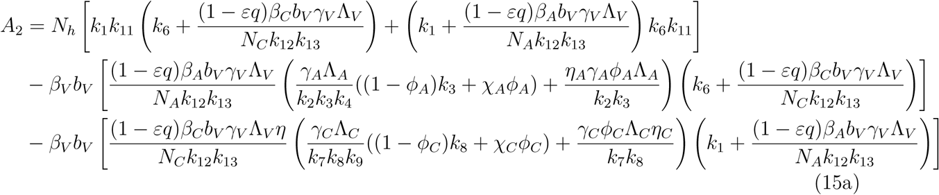
 A2 < 0 if ℛVℛA > 1 and ℛVℛC, A2 > 0 if ℛVℛA < 1 and ℛVℛC < 1


 A3 > 0 if ℛv(ℛA + ℛC) < 1
A3 < 0 if ℛv(ℛA + ℛC) < 1
The model (1) has a unique endemic(positive) equilibrium for the special case when ω = ωC = α = 0 whenever ℛE > 1
Proof:(Proof of Lemma 5)
For model (1), let
(x1 = SA, x2 = EA, x3 = IAM, x4 = IAS, x5 = RA, x6 = R, x7 = SC, x8 = EC, x9 = ICM, x10 = ICS, x11 = RC, x12 = Q, x13 = SV, x14 = EV, x15 = IV).
Thus, the model can be written as
 Consider the case when
  is chosen as the bifurcation parameter. Solving for
  from ℛE = 1 gives
 The Jacobian J (ξ*) of the transformed system (17) evaluated at the disease-free equilibrium with
  gives
gives
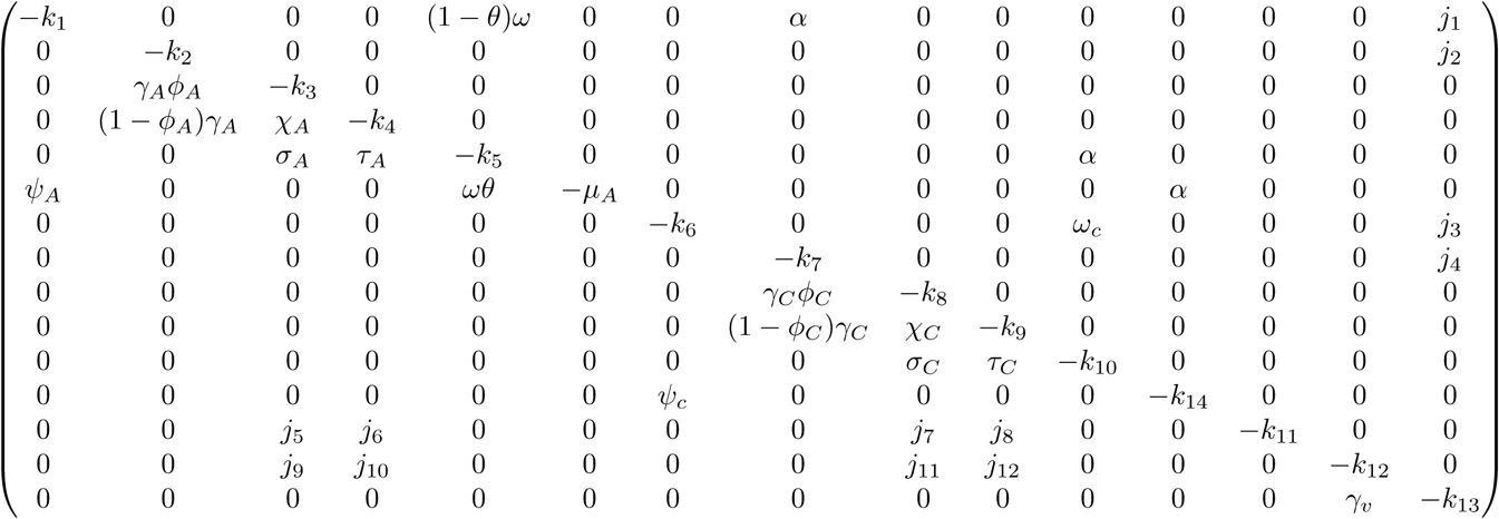 where,
 The right eigen vector of J (ξ*) is given by w = (w1, w2, …w15)T, where
 Where
Where
 Similarly,
  has a left eigenvector v = (v1, v2, …, v15), where
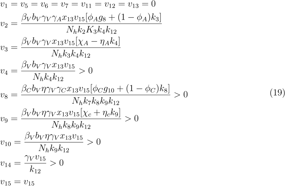 Where
Where
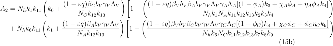
g8 = χA ηAk4, g10 = χC ηCk9, g11 = ϕAηAk4 + k3(1 − ϕA) + χAϕA, g12 = ϕCηCk9 + g3
The associated non-zero partial derivatives of system (17) evaluated at the DFE gives the associated bifurcation coefficients a and b defined by
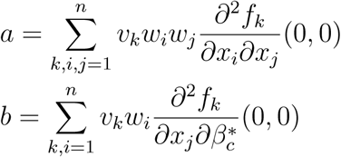 which gives
 . where
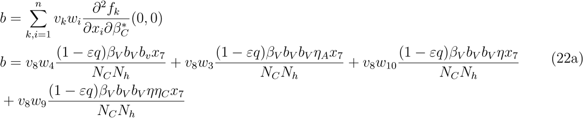
 . Since the bifurcation coefficient is positive. It follows from theorem 2 of ([16]) that the transformed model (17) will undergo a backward bifurcation if the bifurcation coefficient a is positive. The phenomenon of backward bifurcation examines the scenario where a stable DFE coexist with a stable EEP when the associated reproduction number is less than unity.
The epidemiological implication of the backward bifurcation of the model (1) is that the classical requirement of the reproduction number being less than unity becomes only a necessity, but not sufficient condition for malaria control. However, if we set ω(1 − θ) = ωC = ηA = α = 0 in the expression for a in (20b), the bifurcation parameter becomes negative. Thus, it follows from the a Castillo Chavez theorem in [16], that model (1) does not undergo the phenomenon of backward bifurcation if ω(1 − θ) = ωC = ηA = α = 0.
Proof:(Proof of Lemma 6)
To prove the global asymptotic stability of DFE we use a previously described approach in [13]. Let X = (SA, RA, R, SC, RC, Q, SV) and Z = (EA, IAM, IAS, EC, ICM, ICS, EV, IV) and writing the model equation (1) in the form
 , where EA, IAM = IAS = EC= ICM = ICS = EV = IV =0 with F (X, 0) being the RHS of
  and G(X, Z) the RHS of
Next, consider the reduced system:  given as
 be an equilibrium of the reduced system (23), we now show that X* is a globally stable equilibrium in D by solving equations (23) and taking limit as t → ∞
Solving for SA(t) gives
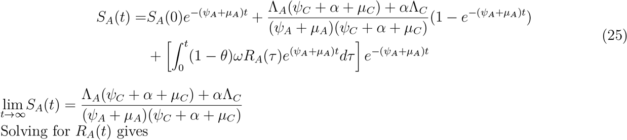

 Solving for RA(t) and substituting the value of SA(t) in the expression obtained gives
 Solving for SC (t) gives


 taking limit of SV (t) as t → ∞ givesV

The asymptotic dynamics are independent of initial conditions in D. Hence, the solutions of (23) converge globally in D. According to previous study [16] it is required to show that G(X, Z) satisfies the two stated conditions
G(X, 0) = 0 and
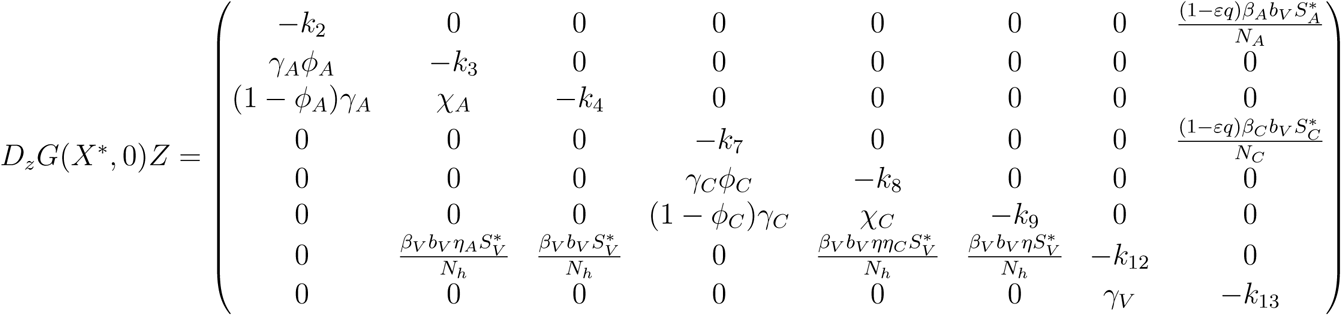
G(X, Z) = DzG(X*, 0)Z − Ĝ (X, Z), Ĝ (X, Z) ≥ 0 where
 DzG(X*, 0) is the Jacobian of G(X, Z) taken with respect to the infected classes and evaluated at (X*, 0).
 and
and
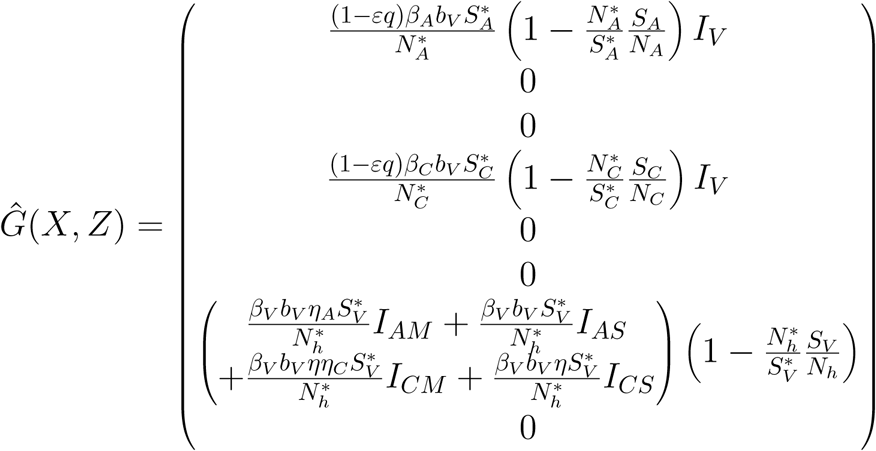 Since we have
 In D,
In D,  and thus
If the human population is at equilibrium, we have
 ; thus Ĝ (X, Z) 0. Therefore, the DFE is globally asymptotically stable by the theorem in [16].
Proof:(Proof of Lemma 7)
Suppose ℛE > 1 then the existence of the endemic equilibrium point is guaranteed. Using the common quadratic Lyapunov function,
 As formerly illustrated [20], we consider a Lyapunov function with the following state variables
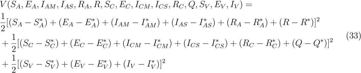 Now, differentiating (33) along the solution curve of (32) gives
 from (32), it implies that
 Plugging (34) to (35) gives
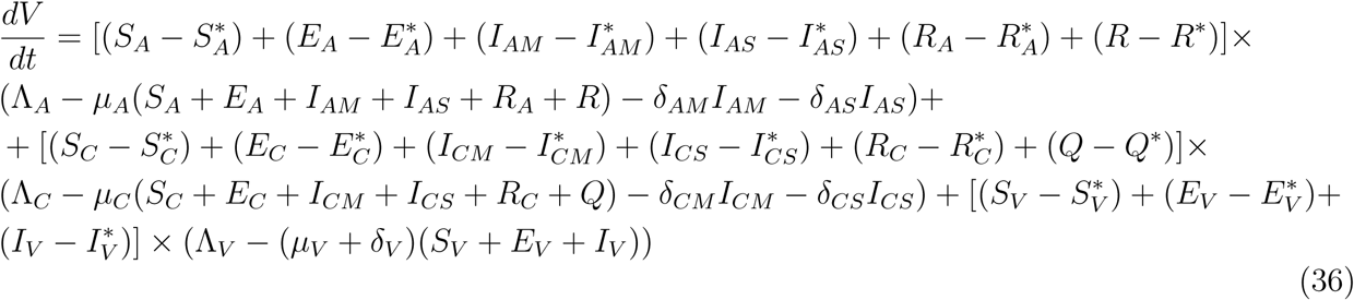 Now assuming,
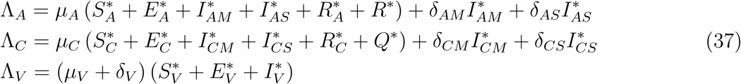 Substituting (37) into (36)
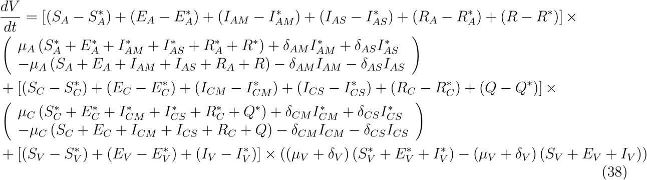
 This implies that
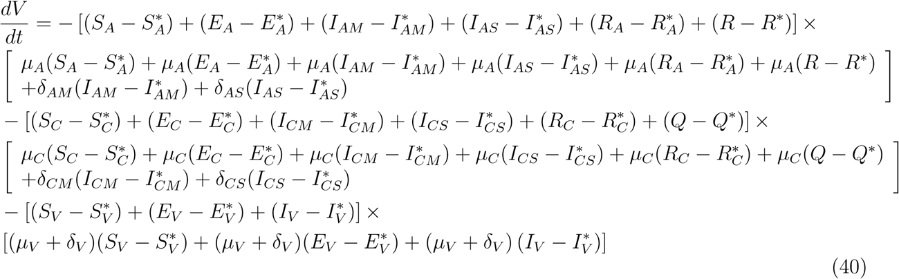 This shows that
  is negative and
  if and only if
 Additionally, every solution of (1) with the initial conditions approaches ξ** as t → ∞.
Therefore, the largest compact invariant set in
 is a singleton set {ξ**}
Therefore, from Lassalle’s invariant principle [21], it implies that the endemic equilibrium ξ** is globally asymptotically stable in D whenever ℛE > 1
References


