Transcriptome-Wide Root Causal Inference

Eric V. Strobl; Eric R. Gamazon

doi:10.1101/2024.07.22.24310837

ABSTRACT

Root causal genes correspond to the first gene expression levels perturbed during pathogenesis by genetic or non-genetic factors. Targeting root causal genes has the potential to alleviate disease entirely by eliminating pathology near its onset. No existing algorithm discovers root causal genes from observational data alone. We therefore propose the Transcriptome-Wide Root Causal Inference (TWRCI) algorithm that identifies root causal genes and their causal graph using a combination of genetic variant and unperturbed bulk RNA sequencing data. TWRCI uses a novel competitive regression procedure to annotate cis and trans-genetic variants to the gene expression levels they directly cause. The algorithm simultaneously recovers a causal ordering of the expression levels to pinpoint the underlying causal graph and estimate root causal effects. TWRCI outperforms alternative approaches across a diverse group of metrics by directly targeting root causal genes while accounting for distal relations, linkage disequilibrium, patient heterogeneity and widespread pleiotropy. We demonstrate the algorithm by uncovering the root causal mechanisms of two complex diseases, which we confirm by replication using independent genome-wide summary statistics.

1 Introduction

Genetic and non-genetic factors can influence gene expression levels to ultimately cause disease. Root causal gene expression levels – or root causal genes for short – correspond to the initial changes to gene expression that ultimately generate disease as a downstream effect¹. Root causal genes differ from core genes that directly cause the phenotype and thus lie at the end, rather than at the beginning, of pathogenesis². Root causal genes also generalize driver genes that only account for the effects of somatic mutations primarily in protein coding sequences in cancer³.

Discovering root causal genes is critical towards identifying drug targets that modify disease near its pathogenic onset and thus mitigate downstream pathogenesis in its entirety⁴. The problem is complicated by the existence of complex disease, where the causal effects of the root causal genes may differ between patients even within the same diagnostic category. However, the recently defined omnigenic root causal model posits that only a few root causal genes initiate the vast majority of downstream pathology in each patient¹. We thus more specifically seek to identify personalized root causal genes specific to any given individual.

Only one existing algorithm accurately identifies personalized root causal genes¹, but the algorithm requires access to genome-wide Perturb-seq data, or high throughput perturbations with single cell RNA sequencing readout^{5, 6}. Perturb-seq is currently expensive and difficult to obtain in many cell types. We instead seek a method that can uncover personalized root causal genes directly from widespread observational (or non-experimental) datasets.

We make the following contributions in this paper:

We introduce the conditional root causal effect (CRCE) that measures the causal effect of the genetic and non-genetic factors, which directly affect a gene expression level, on the phenotype.
We propose a novel strategy called Competitive Regression that provably annotates both cis and trans-genetic variants to the gene expression level or phenotype they directly cause without conservative significance testing.
We create an algorithm called Trascriptome-Wide Root Causal Inference (TWRCI) that uses the annotations to reconstruct a personalized causal graph summarizing the CRCEs of gene expression levels from a combination of genetic variant and bulk RNA sequencing observational data.
We show with confirmatory replication that TWRCI identifies only a few root causal genes that accurately distinguish subgroups of patients even in complex diseases – consistent with the omnigenic root causal model.

We provide an example of the output of TWRCI in Figure 1. TWRCI annotates both cis and trans genetic variants to the expression level or phenotype they directly cause. We prove that the direct causal annotations allow the algorithm to uniquely reconstruct the causal graph between the gene expression levels that cause the phenotype as well as estimate their CRCEs. The algorithm summarizes the CRCEs in the graph by weighing and color-coding each vertex, where vertex size correlates with magnitude, green induces disease and red prevents disease. TWRCI thus provides a succinct summary of root causal genes and their root causal effect sizes specific to a given patient using observational data alone. TWRCI outperforms combinations of existing algorithms across all subtasks: annotation, graph reconstruction and CRCE estimation. No existing algorithm performs all subtasks simultaneously.

Figure 1.

Toy example of a root causal mechanism inferred by TWRCI for a specific patient. Rectangles denote sets of genetic variants, potentially in linkage disequilibrium even between sets. Each set of variants directly causes a gene expression level in or the phenotype Y . Larger lettered vertices denote larger CRCE magnitudes and colors refer to their direction – green is a positive CRCE and red is negative. TWRCI simultaneously annotates, reconstructs and estimates the CRCEs.

2 Results

2.1 Overview of TWRCI

2.1.1 Setup

We seek to identify not just causal but root causal genes. We must therefore carefully define the generative process. We consider a set of variants S, the transcriptome and the phenotype Y. We represent the generative causal process using a directed graph like in Figure 2 (a), where the variants cause the transcriptome, and the transcriptome causes the phenotype. Directed edges denote direct causal relations between variables. In practice, the sets S and contain millions and thousands of variables, respectively. As described in Methods 4.2, we cannot measure the values of X exactly using RNA sequencing but instead measure values corrupted by Poisson measurement error and batch effects.

Figure 2.

Overview of the TWRCI algorithm. (a) We redraw Figure 1 in more detail. We do not have access to the underlying causal graph in practice. (b) TWRCI first performs variable selection by only keeping variants and gene expression levels correlated with Y (and their common cause confounders) as shown in black. (c) The algorithm then uses Competitive Regression to find the variants that directly cause Y in orange. (d) TWRCI iteratively repeats Competitive Regression for each gene expression level as well – again shown in orange. (e) The algorithm next performs causal discovery to identify the causal relations between the gene expression levels and the phenotype in blue. (f) Finally, TWRCI weighs each vertex by the magnitude of Γ_i and color codes the vertex by its direction (green is positive, red is negative). TWRCI thus ultimately recovers a causal graph like the one shown in Figure 1.

2.1.2 Variable Selection

Simultaneously handling millions of variants and thousands of gene expression levels currently requires expensive computational resources. Moreover, most variants and gene expression levels do not inform the discovery of root causal genes for a particular phenotype Y . The Transcriptome-Wide Root Causal Inference (TWRCI) thus first performs variable selection by eliminating variants and gene expression levels unnecessary for root causal inference.

TWRCI first identifies variants T ⊆ S associated with Y using widely available summary statistics at a liberal α threshold, such as 5e-5, in order to capture many causal variants. The algorithm then uses individual-level data – where each individual has variant data, bulk gene expression data from the relevant tissue and phenotype data (variant-expression-phenotype) – to learn a regression model predicting X from T. TWRCI identifies the subset of expression levels that it can predict better than chance. We refer the reader to Methods 4.4.2 for details on the discovery of additional nuisance variables required to mitigate confounding. We prove that retains all of the causes of Y in.

2.1.3 Annotation by Competitive Regression

We want to annotate both cis and trans-variants to the gene expression level that they directly cause in . We also want to annotate variants to the phenotype Y in order to account for horizontal pleiotropy, where variants bypass and directly cause Y . TWRCI achieves both of these feats through a novel process called Competitive Regression.

TWRCI accounts for horizontal pleiotropy by applying Competitive Regression to the phenotype. We do not restrict the theoretical results detailed in Methods to linear models, but linear models trained on genotype data currently exhibit competitive performance^{7, 8}. TWRCI therefore trains linear ridge regression models predicting Y from without imposing Gaussian distributions; let γ_Yi refer to the coefficient for T_i in the regression model. Similarly, let Δ_−Yi correspond to the matrix of coefficients for T in the regression models predicting (but not Y) from T; notice that we have not conditioned on the gene expression levels in this case. If T_i directly causes Y, then it will predict Y given (i.e., γ_Yi will be non-zero), but T_i will not predict any gene expression level given T \ T_i (i.e., max_i |Δ_−Yi | will be zero). Conversely, if γ_Yi deviates away from zero even after conditioning on gene expression such that |γ_Yi | ≥ max_i |Δ_−Yi | – i.e., γ_Yi “beats” Δ_−Yi in a competitive process – then TWRCI annotates T_i to Y (Figure 2 (c)).

We prove in Methods 4.4.3 that Competitive Regression successfully recovers the direct causes of Y, denoted by S_Y ⊆ T, so long as Y is a sink vertex that does not cause any other variable. We also require analogues of two standard assumptions used in instrumental variable analysis: relevance and exchangeability⁹. In this paper, relevance means that at least one variant in T directly causes each gene expression level in ; the assumption usually holds because T contains orders of magnitude more variants than entries in . On the other hand, exchangeability assumes that T and other sets of direct causal variants not in T share no latent confounders (details in Methods 4.4.2); this assumption holds approximately due to the weak causal relations emanating from variants to gene expression and the phenotype. Exchangeability also weakens as T grows larger.

We further show that Competitive Regression can recover S_i ⊆ T, or the direct causes of in T, when causes Y and turns into a sink vertex after removing Y from consideration (Methods 4.4.4). As a result, TWRCI removes Y and appends it to the empty ordered set K to ensure that some is now a sink vertex. We introduce a statistical criterion in Methods 4.4.4 that allows TWRCI to find the sink vertex after the removal of Y . TWRCI then annotates S_i to again using Competitive Regression (Figure 2 (d)), removes R_i from R and appends R_i to the front of K. The algorithm iterates until it has removed all variables from R ∪Y and placed them into the causal order K.

2.1.4 Causal Discovery and CRCE Estimation

Annotation only elucidates the direct causal relations from variants to gene expression, but it does not recover the causal relations between gene expression or the causal relations from gene expression to the phenotype. We want TWRCI to recover the entire biological mechanism from variants all the way to the phenotype.

TWRCI thus subsequently runs a causal discovery algorithm with the causal order K to uniquely identify the causal graph over (Figure 2 (e)). The algorithm also estimates the personalized or conditional root causal effect (CRCE) of gene expression levels that cause Y : where we choose carefully to ensure that the second equality holds (Methods 4.3). The CRCE Γ_i of thus measures the causal effect of the genetic factors S _i and the non-genetic factors E_i on Y that perturb first. The CRCE values differ between patients, so TWRCI can recover different causal graphs by weighing each vertex according to the patient-specific CRCE values Γ= γ (Figure 2 (f)). The gene is a personalized root causal gene if |γ_i | > 0. The omnigenic root causal model posits that |γ| ≫ 0 for only a small subset of genes in each patient even in complex disease.

2.2 TWRCI accurately annotates, reconstructs and estimates in silico

No existing algorithm recovers personalized root causal genes from observational data alone. However, existing algorithms can annotate variants using different criteria and reconstruct causal graphs from observational data. We therefore compared TWRCI against state of the art algorithms in annotation and causal graph reconstruction using 60 semi-synthetic datasets with real variant data but simulated gene expression and phenotype data (Methods 4.6).

Many different annotation methods exist with different objectives. Most methods nevertheless annotate variants by at least considering proximity to the TSS, with the hope that variants near a TSS of a gene will directly affect that gene’s expression level; for example, a variant in an exon of the gene may compromise its mRNA stability, while a variant in the promoter may affect its transcription rate. We thus compare a diverse range of methods in direct causal annotation, or assigning variants to the gene expression levels they directly cause. This criterion accommodates other annotation objectives from a mathematical perspective as well – solving direct causation automatically solves causation, colocalization and correlation as progressively more relaxed cases. We in particular compare nearest TSS, a one mega-base cis-window¹, the causal transcriptome-wide association study (cTWAS)¹⁰, the maximally correlated gene within the cis-window (cis-eQTL)¹¹, colocalization with approximate Bayes factors (ABF)¹², and colocalization with Sum of SIngle Effects model (SuSIE)¹³. We then performed causal graph reconstruction using SIGNET^{14, 15}, RCI¹⁶, GRCI¹⁷ and the PC algorithm^{18, 19}. We evaluated TWRCI against all combinations of annotation and graph reconstruction methods. See Methods 4.5 and 4.8 for a detailed description of comparator algorithms and evaluation metrics, respectively. All statements about empirical results mentioned below hold at a Bonferroni corrected threshold of 0.05 divided by the number of comparator algorithms according to two-sided paired t-tests.

We first summarize the accuracy results for annotation of direct causes only. All existing annotation algorithms utilize heuristics such as location, correlation or colocalization to infer causality. Only TWRCI provably identifies the direct causes of each gene expression level (Theorem 1 in Methods 4.4.6). Empirical results corroborate this theoretical conclusion. TWRCI achieved the highest accuracy as assessed by Matthew’s correlation coefficient (MCC) to the true direct causal variants of each gene expression level and phenotype (Figure 3 (a) left). The algorithm also ranked the ground truth direct causal variants the highest by assigning the ground truth causal variants larger regression coefficient magnitudes than non-causal variants (Figure 3 (a) right). Both TWRCI and cTWAS account for horizontal pleiotropy, but TWRCI again outperformed cTWAS even when we only compared the true and inferred variants that directly cause the phenotype using MCC and the normalized rank (Figure 3 (b)). We conclude that TWRCI annotated the genetic variants to their direct effects most accurately.

Figure 3.

Synthetic data results in terms of (a) direct causal annotation, (b) annotation focused on horizontal pleiotropy only, (c) graph reconstruction, (d) combined annotation and graph reconstruction, and (e) CRCE estimation accuracy. Four of the graphs summarize two evaluation metrics. Arrows near the y-axis denote whether a higher (upward arrow) or a lower (downward arrow) score is better. We do not plot the results of cis-eQTL and SuSIE in (d) due to much worse performance. Error bars correspond to 95% confidence intervals. The cis-window and cTWAS algorithms have the exact same CRCE estimates in (e) because accounting for horizontal pleiotropy in cTWAS does not change the conditioning set D in Equation (1); we thus denote cis-Window and cTWAS as Win/cT for short. TWRCI in purple outperformed all algorithms across all nine evaluation metrics.

We obtained similar results with causal graph reconstruction. TWRCI obtained the best performance according to the highest MCC and the lowest structural hamming distance (SHD) to the ground truth causal graphs (Figure 3 (c)). We then assessed the performance of combined annotation and graph reconstruction using the mean absolute correlation of the residuals (MACR), or the mean absolute correlation between the indirect causes of a gene expression level and the residual gene expression level obtained after partialing out the inferred direct causes; if an algorithm annotates and reconstructs accurately, then each gene expression level should not correlate with its indirect causes after partialing out its direct causes, so the MACR should attain a small value. TWRCI accordingly achieved the lowest MACR as compared to all possible combinations of existing algorithms (Figure 3 (d)). The cis-eQTL and SuSIE algorithms obtained MACR values greater than 0.3 because many cis-variants did not correlate or colocalize with the expression level of the gene with the nearest TSS; we thus do not plot the results of these algorithms. We conclude that TWRCI used annotations to reconstruct the causal graph most accurately by provably accounting for both cis and trans-variants.

We finally analyzed CRCE estimation accuracy. Computing the CRCE requires access to the inferred annotations and causal graph. We therefore again evaluated TWRCI against all possible combinations of existing algorithms. The CRCE estimates of TWRCI attained the largest correlation to the ground truth CRCE values (Figure 3 (e) left). Further, if an algorithm accurately estimates the components and 𝔼 (Y | D) of the CRCE in Equation (1), then the residual should not correlate with S_i ∩T. TWRCI accordingly obtained the lowest mean absolute correlation of these residuals (MACR) against all combinations of algorithms (Figure 3 (e) right). The cis-eQTL and SuSIE algorithms again attained much worse MACR values above 0.4 because they failed to annotate many causal variants to their gene expression levels. We conclude that TWRCI outperformed existing methods in CRCE estimation. TWRCI therefore annotated, reconstructed and estimated the most accurately according to all nine evaluation criteria. The algorithm also completed within about 4 minutes for each dataset (Supplementary Figure 1).

2.3 Adaptive immunity in COPD

We next ran the algorithms using summary statistics of a large GWAS of COPD²⁰ consisting of 13,530 cases and 454,945 controls of European ancestry. We downloaded individual variant-expression-phenotype data of lung tissue from GTEx²¹ with 96 cases and 415 controls. We also replicated results using an independent GWAS consisting of 4,017 cases and 162,653 controls of East Asian ancestry²⁰. COPD is a chronic inflammatory condition of the airways or the alveoli that leads to persistent airflow obstruction²². Exposure to respiratory infections or environmental pollutants can also trigger acute on chronic inflammation called COPD exacerbations that worsen the obstruction.

2.3.1 Accuracy

We first compared the accuracy of the algorithms in variant annotation, graph reconstruction and CRCE estimation. We can compute the MACR metrics – representing two of the nine evaluation criteria used in the previous section – with real data. We summarize the MACR for simultaneous variant annotation and graph reconstruction averaged over ten nested cross-validation folds in Figure 4 (a). TWRCI achieved the lowest MACR out of all combinations of algorithms within about 5 minutes (Supplementary Figure 2 (b) and (c)). Performance differed primarily by the annotation method rather than the causal discovery algorithm. Conservative annotation algorithms, such as colocalization by SuSIE, again failed to achieve a low MACR because they frequently failed to annotate at least one variant to every gene expression level. MACR values for CRCE estimation followed a similar pattern (Figure 4 (b)) because accurate annotation and reconstruction enabled accurate downstream CRCE estimation.

Figure 4.

Results for COPD. (a) TWRCI outperformed all other combinations of algorithms in direct causal annotation and graph reconstruction by achieving the lowest MACR; error bars correspond to one standard error of the mean in accordance with the one standard error rule of cross-validation²⁶. (b) TWRCI similarly achieved the lowest MACR for CRCE estimation. (c) Silver standard genes exhibited the smallest correlation with the phenotype after partialing out the root causal genes inferred by TWRCI. (d) More than 35% the causal variants exhibited horizontal pleiotropy. TWRCI annotated the remaining causal variants to three gene expression levels. (e) TWRCI assigned approximately 84% of the causal variants to genes located on different chromosomes. Most causal variants annotated to a gene on the same chromosome fell within a one megabase distance from the TSS (blue, left). The average magnitude of the regression coefficients decreased slowly with increasing distance starting from about 100 kilo-bases from the TSS (red, right); the dotted line again corresponds to variants on different chromosomes. (f) The COPD-wide causal graph revealed multiple HLA type II genes as root causal. (g) UMAP dimensionality reduction revealed three clusters of COPD patients well-separated from the healthy controls. The directed graphs highlighted different root causal genes within each of those three clusters. Finally, bar graphs revealed different mean gene expression levels relative to healthy controls in each cluster; error bars denote 95% confidence intervals in this case.

We next followed^{10, 23} and downloaded a set of silver standard genes causally involved in COPD from the KEGG database (hsa04660)^{24, 25}. Nearly all of the silver standard genes are causal but not root causal for COPD. If an algorithm truly identifies root causal genes, then partialing out the root causal genes from all of the downstream non-root causal genes and the phenotype should explain away the vast majority of the causal effect between the non-root causal genes and the phenotype according to the omnigenic root causal model. We therefore computed another MACR metric, the mean absolute correlation between the residuals of the silver standard genes and the residuals of the phenotype after removing the inferred root causal genes. TWRCI again obtained the lowest MACR value (Figure 4 (c)). We conclude that TWRCI identified the root causal genes most accurately according to known causal genes in COPD.

2.3.2 Horizontal pleiotropy and trans-variants

We studied the output of TWRCI in detail to gain insight into important issues in computational genomics. Previous studies have implicated the existence of widespread horizontal pleiotropy in many diseases²⁷. TWRCI can annotate variants directly to the phenotype, so we can use TWRCI to assess for the existence of widespread pleiotropy. The variable selection step of TWRCI identified fourteen gene expression levels surviving false discovery rate (FDR) correction at a liberal 10% threshold; three of these levels ultimately caused the phenotype, including HLA-DRB6, HLA-DQA1 and HLA-DQB1. TWRCI annotated 35% of the variants that cause COPD directly to the phenotype, despite competition for variants between the phenotype and the three gene expression levels (Figure 4 (d)). Many variants thus directly cause COPD by bypassing expression. We conclude that TWRCI successfully identified widespread horizontal pleiotropy in COPD. In contrast, cTWAS failed to identify any variants that bypass gene expression because all variants had very small effects on the phenotype, especially after accounting for gene expression; as a result, no variants ultimately had a posterior inclusion probability greater than 0.8 according to cTWAS.

TWRCI annotates both cis and trans-variants, so we examined the locations of the annotated variants relative to the TSS for each of the three causal genes. Most of the variants lying on the same chromosome as the TSS fell within a one megabase distance from the TSS (Figure 4 (e) blue). However, 84% of the variants were located on different chromosomes. We thus compared the variants annotated to causal genes by TWRCI against a previously published list of trans-eQTLs associated with any phenotype in a large-scale search²⁸ (Methods 4.7.3). Variants annotated by TWRCI were located 5.55 times closer to trans-eQTLs than expected by chance (10,000 permutations, P < 0.001, 95% CI [5.49,5.60]). We next examined the effect sizes of the variants that cause the phenotype. We regressed the phenotype on variants inferred to directly or indirectly cause the phenotype using linear ridge regression. We then computed the moving average of the magnitudes of the regression coefficients over different distances from the TSS. The magnitudes decreased slowly with increasing distance starting from about 100 kilo-bases from the TSS (Figure 4 (e) red). However, the magnitudes for variants located on different chromosomes did not converge to zero (dotted line). We thus conclude that trans-variants play a significant role in modulating gene expression to cause COPD.

2.3.3 Root Causal Mechanism

We next analyzed the output of TWRCI to elucidate the root causal mechanism of COPD. The pathogenesis of COPD starts with inhaled irritants that trigger an exaggerated and persistent activation of inflammatory cells such as macrophages and CD4+ T cells²². These cells in turn regulate a variety of inflammatory mediators that promote alveolar wall destruction, abnormal tissue repair and mucous hypersecretion obstructing airflow. The root causal genes of COPD therefore likely involve genes mediating the sustained activation of inflammation.

Three of the fourteen gene expression ultimately caused the COPD phenotype in the causal graph reconstructed by TWRCI (Figure 4 (f)). The graph contained three HLA class II genes that present extracellular peptide antigens to CD4+ T cells in the adaptive immune response²⁹. Subsequent activation of T cell receptors regulates a variety of inflammatory mediators and cytokines³⁰. The recovered causal graph thus implicates the adaptive immune system as the root causal mechanism sustaining chronic inflammation in COPD. TWRCI replicated these results by again discovering multiple HLA class II genes in an independent GWAS dataset composed of patients of East Asian ancestry (Supplementary Figure 3 (a)).

We next used the personalized CRCE estimates to dissect the heterogeneity of COPD. We performed UMAP dimensionality reduction³¹ on the gene expression levels determined to cause the phenotype. Hierarchical clustering with Ward’s method³² yielded four clear clusters of patients with COPD (Figure 4 (g)) according to the elbow method on the sum of squares plot (Supplementary Figure 2 (a)). UMAP differentiated three of the COPD clusters from healthy controls, each with different mean CRCE estimates (Figure 4 (g) directed graphs). HLA-DQB1 had a large positive CRCE in cluster one, while the other two genes had large negative CRCEs in the other two clusters. The CRCEs correlated negatively with the marginal levels of HLA-DRB6 and HLA-DQB1 (Figure 4 (g) bar graphs). We conclude that TWRCI differentiated multiple subgroups of patients consistent with the pathobiology of COPD – likewise for the replication dataset (Supplementary Figure 3 (b) to (d)).

2.4 Oxidative stress in ischemic heart disease

We also ran the algorithms on summary statistics of ischemic heart disease (IHD) consisting of 31,640 cases and 187,152 controls from Finland³³. We used variant-expression-phenotype data of whole blood from GTEx²¹ with 113 cases and 547 controls. We used whole blood because IHD arises from narrowing or obstruction of the coronary arteries most commonly secondary to atherosclerosis with transcription products released into the bloodstream³⁴. We replicated the results using an independent set of GWAS summary statistics from 20,857 cases and 340,337 controls from the UK Biobank³⁵.

2.4.1 Accuracy

We compared the algorithms in variant annotation, graph reconstruction and CRCE estimation accuracy. TWRCI achieved the lowest MACR in both cases (Figure 5 (a) and (b)) within about 90 minutes (Supplementary Figure 4 (b) and (c)). Cis-eQTLs and colocalization with SuSIE failed to annotate many variants because many trans-variants again predicted gene expression. We obtained similar results with a set of silver standard genes downloaded from the KEGG database (hsa05417), where TWRCI outperformed all other algorithms by a very large margin (Figure 5 (c)).

Figure 5.

Results for IHD. (a) TWRCI again outperformed all other algorithms in combined annotation and graph reconstruction by achieving the lowest MACR. (b) TWRCI also estimated the CRCEs most accurately relative to all possible combinations of the other algorithms. (c) TWRCI outperformed all other algorithms with a silver standard set of genes causally involved in atherosclerosis. (d) TWRCI annotated variegated numbers of variants to five causal expression levels as well as the phenotype. (e) Nearly all of the annotated variants were located distal to the TSS (blue), and the magnitudes of their causal effects again decreased gradually with increasing distance from the TSS (red). (f) TWRCI estimated the largest mean CRCE for MRPL1 by far. (g) UMAP dimensionality reduction identified two clusters of patients clearly separated from healthy controls. The mean CRCE of MRPL1 remained the largest in both clusters, but TPT1 ASO also had a large negative mean CRCE in the second cluster

2.4.2 Horizontal pleiotropy and trans-variants

The genetic variants predicted 27 gene expression levels at an FDR threshold of 10% with five genes inferred to cause the phenotype. We plot the five genes in the directed graph recovered by TWRCI in Figure 5 (f). TWRCI sorted approximately 12-23% of the causal variants to each of the five genes (Figure 5 (d)). Moreover, TWRCI annotated approximately 15% of the causal variants directly to the phenotype supporting widespread horizontal pleiotropy in IHD. In contrast, cTWAS again did not detect any variants that directly cause the phenotype with a posterior inclusion probability greater than 0.8.

We analyzed the inferred causal effects of cis and trans-variants. Only 8.8% of the annotated variants were located on the same chromosome, and those on the same chromosome were often located over 10 megabases from the TSS (Figure 5 (e) blue). Moreover, variants annotated by TWRCI were located 4.19 times closer to a published list of trans-eQTLs than expected by chance (10,000 permutations, P < 0.001, 95% CI [4.16,4.22]). The magnitudes of the regression coefficients decreased gradually to 0.002 – rather than to zero – as the distance from the TSS increased (Figure 5 (e) red). We conclude that trans-variants also play a prominent role in IHD.

2.4.3 Root Causal Mechanism

We next examined the root causal genes of IHD. Sites of disturbed laminar flow and altered shear stress trap low-density lipoprotein (LDL) in atherosclerosis. Reactive oxygen species then oxidize LDL and stimulate an inflammatory response³⁶. T cells in turn stimulate macrophages that ingest the oxidized LDL. The macrophages then develop into lipid-laden foam cells that form the initial fatty streak of an eventual atherosclerotic plaque. We therefore expect the root causal genes of IHD to at least involve oxidative stress.

The mitochondrial gene MRPL1 indeed had the largest mean CRCE across all IHD patients by far (Figure 5 (f)). MRPL1 encodes a mitochondrial ribosomal protein that assists in the synthesis of complex proteins involved in the respiratory chain³⁷. Deficiency of MRPL1 can lead to increased oxidative stress. TPT1 is a molecular chaperone that promotes cell survival by reducing oxidative stress³⁸. We conclude that TWRCI accurately detected root causal genes expected from the known pathobiology of IHD. Finally, TWRCI rediscovered MRPL1 in a second independent GWAS dataset (Supplementary Figure 5 (a)).

We next ran UMAP dimensionality reduction on all of the causal genes of IHD discovered by TWRCI. Hierarchical clustering revealed three clusters of IHD patients (Supplementary Figure 4 (a)), two of which lied distal to the cluster of healthy controls (Figure 5 (g) embedding). The MRPL1 gene retained the largest mean CRCE in both clusters (Figure 5 (g) directed graphs). TWRCI likewise replicated the large mean CRCE estimates for MRPL1 in both clusters in the independent GWAS dataset (Supplementary Figure 5 (b) and (c)). However, TPT1 antisense oligonucleotide (TPT1 ASO) also protected against IHD in the second cluster. The CRCE estimates of MRPL1 and TPT1 ASO both decreased with increasing levels of the genes (Figure 5 (g) bar graphs) consistent with their known protective effects again oxidative stress. TWRCI thus detected root causal genes involved in oxidative stress even within patient subgroups.

3 Discussion

We introduced the CRCE of a gene, a measure of the causal effect of the genetic and non-genetic factors that directly cause a gene expression level on a phenotype. We then created the TWRCI algorithm that estimates the CRCE of each gene after simultaneously annotating variants and reconstructing the causal graph for improved statistical power. TWRCI annotates, reconstructs and estimates more accurately than alternative algorithms across multiple semi-synthetic and real datasets. Applications of TWRCI to COPD and IHD revealed succinct sets of root causal genes consistent with the known pathogenesis of each disease, which we verified by replication. Furthermore, clustering delineated patient subgroups whose pathogeneses were dictated by different root causal genes.

Our experimental results highlight the importance of incorporating trans-variants in statistical analysis. TWRCI annotated many variants distal to the TSS of each gene. These trans-variants improved the ability of the algorithm to learn models of gene regulation consistent with the correlations in the data according to the MACR criteria. Moreover, variants annotated by TWRCI were located 4-6 times closer to the positions of a previously published list of trans-eQTLs than expected by chance²⁸. In contrast, nearest TSS, cis-windows, cTWAS, cis-eQTLs and the colocalization methods all rely on cis-variants that did not overlap with many GWAS hits both in the COPD and IHD datasets. Most GWAS hits likely lie distal to the TSSs in disease due to natural selection against cis-variants with large causal effects on gene expression³⁹. As a result, algorithms that depend solely on cis-variants can fail to detect a large proportion of variants that cause disease in practice.

TWRCI detected widespread horizontal pleiotropy accounting for 15-35% of the causal variants in both the COPD and IHD datasets. Previous studies have detected horizontal pleiotropy in around 20% of causal variants even after considering thousands of gene expression levels as well²⁷. Moreover, many of the variants annotated to the phenotype by TWRCI correlated with gene expression (Supplementary Figures 2 (d) and 4 (d)). Accounting for widespread horizontal pleiotropy thus mitigates pervasive confounding between gene expression levels and the phenotype.

The cTWAS algorithm did not detect widespread pleiotropy in the real datasets. The algorithm also underperformed TWRCI in the semi-synthetic data, even when we restricted the analyses to variants that directly cause the phenotype. We obtained these results because cTWAS relies on the SuSIE algorithm to identify pleiotropic variants. However, pleiotropic variants usually exhibit weak causal relations to the phenotype, so most of these variants do not achieve a large posterior inclusion probability in practice. Algorithms that depend on absolute measures of certainty, such as posterior probabilities or p-values, miss many causal variants with weak causal effects in general. TWRCI therefore instead annotates variants by relying on relative certainty via a novel process called Competitive Regression, which we showed leads to more consistent causal models across multiple metrics.

We re-emphasize that TWRCI is the only algorithm that accurately recovers root causal genes initiating pathogenesis. Other methods such as colocalization and cTWAS identify causal genes involved in pathogenesis, regardless of whether the genes are root causal or not root causal. As a result, only TWRCI inferred a few genes with large CRCE magnitudes even in complex diseases. Moreover, genes with non-zero CRCE magnitudes explained away most of the causal effects of the non-root causal genes in the silver standards. Both of these results are consistent with the omnigenic root causal model, or the hypothesis that only a few root causal genes initiate the vast majority of downstream pathology in each patient even in complex disease¹. Note that these root causal genes differ from driver genes and core genes. Root causal genes generalize driver genes by accounting for all of the factors that directly influence gene expression levels across all diseases, rather than just somatic mutations in cancer³. Root causal genes also differ from core genes, or the gene expression levels that directly cause a phenotype, by focusing on the beginning rather than the end of pathogenesis². Root causal genes may affect the expression levels of downstream genes so that many genes are differentially expressed between patients and healthy controls including many core genes. A few root causal genes can therefore increase the polygenicity of the core gene model.

TWRCI provably identifies root causal genes with strong empirical accuracy, but the algorithm carries several limitations. The algorithm cannot accommodate cycles or directed graphs with different directed edges, even though cycles may exist and direct causal relations may differ between patient populations in practice⁴⁰. TWRCI also estimates CRCE values at the patient-specific level, but the CRCEs may also vary between different cell types. Finally, the algorithm uses linear rather than non-linear models to quantify the causal effects of the variants on gene expression or the phenotype. Future work should therefore consider relaxing the single DAG constraint and accommodating non-linear relations. Future work will also focus on scaling the method to millions of genetic variants without feature selection.

In summary, we introduced an algorithm called TWRCI for accurate estimation and interpretation of the CRCE using personalized causal graphs. TWRCI empirically discovers only a few gene expression levels with large CRCE magnitudes even within different patient subgroups of complex disease in concordance with the omnigenic root causal model⁴¹. We conclude that TWRCI is a novel, accurate and disease agnostic procedure that couples variant annotation with graph reconstruction to identify root causal genes using observational data alone.

Data Availability

All datasets analyzed in this study have been previously published and are publicly accessible as described in Methods.

https://github.com/ericstrobl/TWRCI

4 Methods

4.1 Background on Causal Discovery

Causal discovery refers to the process of discovering causal relations from data. We let italicized letters such as Z_i denote a singleton random variable and bold italicized letters such as Z denote sets of random variables. Calligraphic letters such as 𝒵 refer to sets of sets.

We consider a set of P endogenous variables Z. We represent a causal process over Z using a structural equation model (SEM) consisting of a series of deterministic functions: where Pa(Z_i) ⊆ Z \ Z_i denotes the parents, of direct causes, of Z_i and E_i ∈ E an exogenous variable, also called an error or a noise term. We assume that the variables in E are mutually independent. The set Ch(Z_i) refers to the children, or direct effects, of Z_i where Z_j ∈ Ch(Z_i) if and only if Z_i ∈ Pa(Z_j).

We can associate an SEM with a directed graph 𝔾 by a drawing a directed edge from Z_j to Z_i when Z_j ∈ Pa(Z_i). We thus use the words variable and vertex interchangeably. A root vertex in 𝔾 refers to a vertex without any parents, whereas a sink or terminal vertex refers to a vertex without any children. A path between Z₀ and Z_n corresponds to an ordered sequence of distinct vertices ⟨Z₀, …, Z_n⟩ such that Z_i and Z_i+1 are adjacent for all 0 ≤ i ≤ n − 1. In contrast, a directed path from Z₀ to Z_n corresponds to an ordered sequence of distinct vertices ⟨Z₀, …, Z_n⟩ such that Z_i ∈ Pa(Z_i+1) for all 0 ≤ i ≤ n − 1. We say that Z_j is an ancestor of Z_i, and likewise that Z_i is a descendant of Z_j, if there exists a directed path from Z_j to Z_i (or Z_j = Z_i). We collect all ancestors of Z_j into the set Anc(Z_j), and all its non-descendants into the set Nd(Z_j). We write Z_i ∈ Anc (A) when Z_i is an ancestor of any variable in A, and likewise Nd(A) for the non-descendants. The variable Z_j causes Z_i if Z_j is an ancestor of Z_i and Z_j ≠ Z_i. A root cause of Z_i corresponds to a root vertex that also causes Z_i.

A cycle exists in 𝔾 when Z_j causes Z_i and vice versa. A directed acyclic graph (DAG) corresponds to a directed graph without cycles. A collider corresponds to Z_j in the triple Z_i → Z_j ← Z_k. Two vertices Z_i and Z_j are d-connected given W ⊆ Z \ {Z_i, Z_j } if there exists a path between Z_i and Z_j such that no non-collider is in W and all colliders are ancestors ofW. We denote d-connection by for shorthand. The two vertices are d-separated given W, likewise denoted by Z_i𝔾 _d Z_j|W, if they are not d-connected. A path is blocked by W if W contains at least one non-collider on the path or does not contain an ancestor of a collider (or both).

A probability density that obeys an SEM associated with the DAG 𝔾 also factorizes according to the graph:

Any density that factorizes as above obeys the global Markov property, where Z_i and Z_j are conditionally independent given W, or Z_i ╨ Z_j|W if Z_i ╨ _d Z_j|W⁴². A density obeys d-separation faithfulness when the converse holds: if Z_i ╨ Z_j|W, then Z_i ╨ _d Z_j|W.

4.2 Causal Modeling of Variants, Gene Expression and the Phenotype

We divide the set of random variables Z into disjoint sets corresponding to the phenotype Y, q genetic variants S, latent variables L modeling linkage disequilibrium (LD) and m gene expression levels . We model the causal process over Z using the following SEM associated with a DAG 𝔾: where and for any latent variable, any genetic variant, any gene expression level and the phenotype, respectively. In other words, linkage disequilibrium L generates variants S, and variants and gene expression generate other gene expression levels and the phenotype Y (example in Figure 6 (a)). We assume that Y is a sink vertex such that gene expression and variants cause Y but not vice versa.

Figure 6.

(a) An example of a DAG over Z. In (b), the additional vertices X denote counts corrupted by batch B effects and Poisson measurement error. (c) We can also augment the DAG in (a) with root vertex error terms E.

Let S_i denote the direct causes of in S. We require S_i ≠ ∅ for all so that at least one variant directly causes each gene expression level. We also assume that any single variant can only directly cause one gene expression level or the phenotype (but not both). Investigators have reported only a few rare exceptions to this latter assumption in the literature⁴¹. A variant may however indirectly cause many gene expression levels.

We unfortunately cannot measure the exact values of gene expression using RNA sequencing (RNA-seq) technology. Numerous theoretical and experimental investigations have revealed that RNA-seq suffers from independent Poisson measurement error^{43, 44}: where π denotes the mapping efficiency of in batch j . We thus sample Y ∪ S ∪ L ∪ X ∪ B from the DAG like the one shown in Figure 6 (b) in practice, where B denotes the batch. With slight abuse of terminology, we will still call a sink vertex if it has only one child X_i.

We can perform consistent regression under Poisson measurement error. Let denote the library size and let denote the true unobserved total gene expression level weighted by the mapping efficiencies in batch j . Also let and refer to any subset of gene expression levels and variants, respectively. The following result holds:

Lemma 1.

Assume Lipschitz continuity of the conditional expectation for all N ≥ n₀: where C_N ∈ O(1) is a positive constant, and we have taken an outer expectation on both sides. Then almost surely.

We delegate proofs to the Supplementary Materials. Intuitively, approaches as the library size increases, so the above lemma states that accurate estimation of implies accurate estimation of . We can thus consistently estimate any conditional expectation using 𝔼 (Z_i |U,V, B) when the library size approaches infinity. We only apply the asymptotic argument to bulk RNA-seq, where the library size is on the order of at least tens of millions. We henceforth implicitly assume additional conditioning on B whenever regressing to or on bulk RNA-seq data in order to simplify notation.

4.3 Conditional Root Causal Effects

We define the root causal effect of a gene expression level on the phenotype Y . We focus on Equation (3) with the endogenous variables Z and the exogenous variables E. If the error terms E are mutually independent, then we can augment the associated DAG 𝔾 with E by drawing a directed edge from each to its direct effect Z_i (Figure 6 (c)). We denote the resultant graph by 𝔾^′, where we always have and the subscript emphasizes the augmented DAG; if we do not place a subscript, then we refer to the original DAG 𝔾. Only the error terms are root vertices in 𝔾^′, so only exogenous variables that cause Y can be root causes of Y .

The root causal effect of Z_i on Y given the exogenous variables E is the causal effect of its direct causes in E on Y :

The variable Z_i is the first variable in Z affected by , and Z_i may in turn causally affect Y . The exogenous variable models the effects of environmental, epigenetic and other non-genetic factors on Z_i because the set of endogenous variables includes the genetic factors S. The root causal effect is a special case of the conditional root causal effect (CRCE) given the exogenous variables E: where (1) and (2) . The first condition ensures that D does not block any directed path from Z_i to Y . The second ensures that D eliminates any confounding between and Y . The first condition actually implies the second in this case because E are root vertices. If we set D = ∅, then we recover the unconditional root causal effect in Equation (4).

We are however interested in identifying the causal effects of both genetic and non-genetic factors on Y through gene expression with potential confounding between members of S due to LD. We therefore expand the set of exogenous variables to E ∪ S representing the non-genetic and genetic factors, respectively. We define the conditional root causal effect of given the exogenous variables E ∪ S as: where we write to prevent cluttering of notation. The set E_i ∪ S_i thus refers to the direct causes of in E ∪ S. The above conditional root causal effect measures the causal effect of the root vertices E on Y as they pass through E_i ∪ S_i to

We can likewise choose any D such that and . We choose D carefully to satisfy these two conditions as well as elicit favorable mathematical properties by setting , where and . This particular choice of D allows us to write: so that we do not need to recover E_i as an intermediate step. We prove the second equality in Proposition 1 of the Supplementary Materials under exchangeability, or no latent confounding by L between any two entries of ; this union corresponds to a set of sets including T and each entry of { Anc(Y)} in the set. Exchangeability holds approximately in practice due to the weak causal relations emanating from variants to gene expression and the phenotype. Moreover, the assumption weakens with more variants in T. Now the first gene expression level in affected by E_i∪ S_i is . We thus call a root causal gene if also causes Y such that Ψ_i ≠ 0.

We finally focus on the expected version of Ψ_i to enhance computational speed, improve statistical efficiency and overcome Poisson measurement error according to Lemma 1:

The omnigenic root causal model posits that |γ| ≫ 0 for only a small subset of gene expression levels in each patient with Γ= γ. We thus seek to estimate the values γ for each patient. We use the acronym CRCEs to specifically refer to Γ from here on.

4.4 Algorithm

4.4.1 Strategy Overview

We seek to accurately annotate, reconstruct and estimate the CRCEs using (1) summary statistics as well as (2) linked variant-expression-phenotype data. We summarize the proposed Transcriptome-Wide Root Causal Inference (TWRCI) algorithm in Algorithm 1. TWRCI first uses summary statistics to identify variants T associated with the phenotype at a liberal α threshold in Line 1. The algorithm also identifies gene expression levels R ⊆ X predictable by T in Line 1 from the variant-expression-phenotype data. TWRCI then annotates non-overlapping sets of variants to the phenotype in Line 2 and each gene expression level in Line 3 using a novel process called Competitive Regression. Competitive Regression assigns a variant to the phenotype or gene expression level it most strongly predicts, and we prove that annotated variants include all of the direct causes in T. TWRCI identifies the causal ordering K among during the annotation process. The algorithm finally recovers the directed graph uniquely given K in Line 4 and estimates the CRCE of each gene inferred to cause Y using the estimated graph and the annotations 𝒫 in Line 5. TWRCI can thus weigh and color-code each node in that causes Y by the CRCE estimates for each patient. We will formally prove that TWRCI is sound and complete at the end of this subsection.

Algorithm 1

Transcriptome-Wide Root Causal Inference (TWRCI)

4.4.2 Variable Selection

We summarize the variable selection portion of TWRCI in Algorithm 2. TWRCI first reduces the number of variants using summary statistics by only keeping variants with a significant association to the phenotype at a very liberal α threshold (Line 1); we use 5e-5, or a three orders of magnitude increase from the usual threshold of 5e-8. We do not employ clumping or other pre-processing methods that may remove more variants from consideration. Let T denote the variants that survive this screening step so that .

The variable selection algorithm then identifies the gene expression levels predictable by T using the variant-expression-phenotype data in Line 2. We operationalize this step by linearly regressing X on T using half of the samples, and then testing whether the predicted level and the true level X_i linearly correlate in the second half for each X_i ∈ X⁴⁵. This sample splitting procedure ensures proper control of the Type I error rate⁴⁶. We keep gene expression levels R ⊆ X that achieve a q-value below a liberal FDR threshold of 10%⁴⁷. We say that T is relevant if it contains at least one variant that directly causes each member of . We finally repeat the above procedure after regressing out R from X\ R and T in Line 3 in order to identify Ñ, or all parents of in . We call N the set of nuisance variables, since we will need to condition on them, but they do not contain the ancestors of Y . Algorithm 2 formally identifies the necessary ancestors needed for downstream inference:

Lemma 2.

Assume d-separation faithfulness and relevance. Then, (1) the set contains all of the ancestors of Y in , and (2) the set Ñ contains all of the parents of in ,but none of the effects of .

Algorithm 2

Variable Selection

4.4.3 Annotation for Horizontal Pleiotropy

TWRCI next annotates the associated variants T to their direct effects in . The algorithm first annotates a sink vertex and then gradually works its way up the DAG until it annotates the final root vertex.

TWRCI assumes that Y is a sink vertex, so it first annotates to Y . A variant exhibits horizontal pleiotropy if it directly causes Y . We propose a novel competitive regression scheme to annotate all members of T ∩ Pa(Y) = S_Y to Y .

We mildly assume equality in conditional expectation implies equality in conditional distribution and vice versa. Let and likewise Q = R ⋃ Y . We also mildly assume that the following contribution scores exist and are finite: Δ_ij = 𝔼|∂𝔼(Q_i|T)/∂T_j| and , where denotes the non-descendant gene expression levels of in including the parents. The scores correspond to the variable coefficients in linear regression. We use the contribution scores to annotate any T_j ∈ T such that |γ_{Y j} | ≥ max|Δ_Rj | to Y, since this set of variants corresponds to a superset of S_Y by the following result:

Corollary 1.

Under d-separation faithfulness and exchangeability, |γ_{Y j} | ≥ max|Δ_Rj | if and only if T_j ∉ Anc(R) or T_j ∈ Pa(Y) (or both).

The proof follows directly from Lemma 3 in the Supplementary Materials.

The Competitive Regression (CR) algorithm summarized in Algorithm 3 computes the contribution scores in order to annotate variants to Y . Let Δ_−i denote the removal of the i^th row from Δ corresponding to Q_i = Y . We use linear ridge regression to compute Δ_−i in Line 1 and γ_i in Line 2. CR compares the two quantities and outputs the set P_i = {T_j : |γ_{i j} | ≥ max|Δ_{−i j} |}, or a superset of S_i ∩T not including any other variants with children in according to Corollary 1, in Line 3.

Algorithm 3

Competitive Regression (CR)

4.4.4 Annotation and Causal Order

The CR algorithm requires the user to specify a known sink vertex. We drop this assumption by integrating CR into the Annotation and Causal Order (ACO) algorithm that automatically finds a sink vertex at each iteration.

ACO takes R, N,Y, T, P_Y as input as summarized in Algorithm 4. The algorithm constructs a causal ordering over R ∪Y in K by iteratively eliminating a sink vertex from R and appending it to the front of K. ACO also instantiates a list 𝒫 and assigns genetic variants P_i = {T_j : |γ_{i j} | ≥ max|Δ_{−i j} |} ∈ 𝒫 to each gene expression level R_i ∈ R in Lines 8 and 14 using the following generalization of Corollary 1:

Algorithm 4

Annotation and Causal Order (ACO)

Lemma 3.

Assume d-separation faithfulness, relevance and exchangeability. Further suppose that is a sink vertex. Then, |γ_{i j} | ≥ max|Δ_{−i j} | if and only if T_j ∉ Anc(Q \ Q_i) or (or both).

The set P_i is thus again a superset of S_i ∩T, and any additional variants in P_i do not directly cause another gene expression level or the phenotype.

We have thus far assumed that is a sink vertex. However, ACO determines whether is indeed a sink vertex from data using the following result:

Lemma 4.

is a sink vertex if and only if in Line 9 of ACO under d-separation faithfulness, relevance and exchangeability.

ACO practically determines whether any is indeed a sink vertex post variable elimination by first computing the residuals F_i after regressing R on , the nuisance variables Ñ and the identified variants U . A sink vertex has residuals F that are uncorrelated with the variants in T \ (O ∪U_i) in Line 9 by Lemma 4, so ACO can identify the sink vertex in Line 11 as the variable with the smallest absolute linear correlation. The algorithm then appends R_i to the front of K and eliminates R_i from R in Lines 12 and 13, respectively. ACO finally adds U_i to 𝒫 in Line 14, so U_i can be removed from T of the next iteration through O. We formally prove the following result:

Lemma 5.

Under d-separation faithfulness, relevance and exchangeability, ACO recovers the correct causal order K over and (S_i ∩T) ⊆ P_i for all.

4.4.5 Causal Graph Discovery

TWRCI uses the causal order K and the annotations 𝒫 to perform causal discovery. The algorithm runs the (stabilized) skeleton discovery procedure of the Peter-Clark (PC) algorithm to identify the presence or absence of edges between any two gene expression levels (Algorithm 5)^{18, 48}. We modify the PC algorithm so that it tests whether R_i and R_j are conditionally independent given P_i ∪ Ñ and subsets of the neighbors of in in Line 12 to ensure that we condition on all parents of Finally, we orient the edges using the causal order K in Line 19 to uniquely recover the DAG over:

Lemma 6.

Under d-separation faithfulness, relevance and exchangeability, the graph discovery algorithm outputs the true sub-DAG over given a conditional independence oracle, K and 𝒫.

We next include the phenotype Y into the causal graph. We often only have a weak causal effect from gene expression and variants to the phenotype. We therefore choose to detect any causal relation to Y rather than just direct causal relations using Algorithm 6. Algorithm 6 only conditions on in Line 4 to discover both direct and indirect causation in concordance with the following result:

Lemma 7.

Under d-separation faithfulness, relevance and exchangeability, causes Y – and likewise the vertices S_i ∪ E_i cause Y – if and only if .

Algorithm 5

Graph Discovery

Algorithm 6

CRCE Graph Discovery

4.4.6 Conditional Root Causal Effect Estimation

TWRCI finally estimates the CRCEs of the genes that cause Y given the recovered graph and the annotations 𝒫 . We estimate the two conditional expectations in Equation (5) using kernel ridge regression⁴⁹. We embed X_i and using a radial basis function kernel but embed T \ P_i using a normalized linear kernel. We normalize the latter to prevent the linear kernel from dominating the radial basis function kernel, since the variables in T \ P_i typically far outnumber those in.

We now integrate all steps of TWRCI by formally proving that TWRCI is sound and complete:

Theorem 1.

(Fisher consistency) Under d-separation faithfulness, relevance and exchangeability, TWRCI identifies all of the direct causal variants of , the unique causal graph over and the CRCEs of almost surely as N → ∞ with Lipschitz continuous conditional expectations and a conditional independence oracle.

We perform conditional independence testing by correlating the regression residuals of non-linear transformations of the gene expression levels and phenotype⁵⁰. As a result, Lemma 1 also enables accurate conditional independence testing over subsets of , even though we only have access to T ∪ R ∪ N.

4.4.7 Time Complexity

We analyze the time complexity of TWRCI in detail. TWRCI can admit different regression procedures, so we will assume that each regression takes O(c³) time, where c denotes the dimensionality of the conditioning set typically much larger than the sample size n. Most regression procedures satisfy the requirement.

TWRCI first runs Algorithm 2 which requires O(q) time in Line 1 with summary statistics, O(q³m) time in Line 2 with at most m regressions on T, and O(m³ (m + q)) time for at most m + q regressions on in Line 3. Algorithm 2 thus takes O(m⁴ + m³q) + O(q³m) time in total.

TWRCI next annotates to Y using Algorithm 3 which takes O(q³m) + O((m + q)³) time for Lines 1 and 2, respectively. Annotation to Y therefore carries a total time complexity of O(m³q³). TWRCI then runs Algorithm 4. Each iteration of the repeat loop in Line 3 of Algorithm 4 takes O(q³) time for the regression in Line 4 and O(m(m + q)³) time for the at most m regressions in Line 7. The repeat loop iterates at most m times, so Algorithm 4 has a total time complexity of O(m(q³ + m(m + q)³)) = O(m⁵q³).

Algorithm 5 dominates Algorithm 6 in time during the causal graph discovery portion of TWRCI. Algorithm 5 runs in O(m^e (m + q)³) = O(m^e+3q³) time, where e denotes the maximum neighborhood size¹⁸. Finally, CRCE estimation in Line 5 requires O(2m(m + q)³) = O(m⁴q³) time for at most 2m regressions on expression levels and variants. Thus TWRCI in total requires O(m⁴ + m³q) + O(q³m) + O(m³q³) + O(m⁵q³) + O(m^e+3q³) + O(m⁴q³) = O(m⁵q³) + O(m^e+3q³) time. We conclude that the ACO and Graph Discovery sub-algorithms dominate the time complexity of TWRCI.

4.5 Comparators

We compared TWRCI against state of the art algorithms enumerated below.

Annotation

Nearest TSS: annotates each variant to its closest gene according to the TSS.
Cis-window: annotates a variant to a gene if the variant lies within a one megabase window of the TSS. If a variant lies in multiple windows, then we assign the variant to the closest TSS.
Causal transcriptome-wide association study (cTWAS)¹⁰: annotates variants to genes using cis-windows and then accounts for horizontal pleiotropy using the Sum of SIngle Effects (SuSIE) algorithm.
Cis-eQTLs¹¹: annotates a variant to a gene if (1) the variant lies in the cis-window of the gene per above, and (2) the variant correlates most strongly with that gene expression level relative to the other levels.
Colocalization with approximate Bayes factors¹²: annotates each variant to the gene expression level with the highest colocalization probability according to approximate Bayes factors. We could not differentiate this method from cis-windows using the MACR criteria for the real data (Methods 4.8), since the algorithm always assigns higher approximate Bayes factors to cis-variants.
Colocalization with SuSIE^{12, 13}: same as above but with probabilities determined according to SuSIE. We could differentiate this method from cis-windows using the MACR criteria for the real data.

Causal Graph Reconstruction

SIGNET^{14, 15}: predicts gene expression levels from variants using ridge regression and then recovers the genetic ancestors of each expression level by running the adaptive LASSO on the predicted expression levels. The method thus assumes linearity.
RCI¹⁶: assumes a linear non-Gaussian acyclic model⁵¹, and recovers the causal order by maximizing independence between gene expression level residuals obtained from linear regression.
GRCI¹⁷: same as above but assumes an additive noise model⁵² and uses non-linear regression.
PC/CausalCell¹⁹: runs the stabilized PC algorithm^{18, 48} on the gene expression levels using a non-parametric conditional independence test⁵⁰.

4.6 Semi-Synthetic Data

The causal graph reconstruction algorithms all require a variable selection step with gene expression data, since they cannot scale to the tens of thousands of genes with the neighborhood sizes seen in practice^{1, 19}. We therefore assessed the performance of the algorithms independent of variable selection by first instantiating a DAG directly over with p = 30 variables including 29 gene expression levels and a single phenotype. We generated a linear SEM obeying Equation (3) such that for every with E_i ∼ 𝒩 (0, 1/25) to enable detection of weak causal effects from variants. We drew the coefficient matrix β from a Bernoulli(2/(P − 1)) in the upper triangular portion of the matrix and then randomly permuted the ordering of the variables. The resultant DAG has an expected neighborhood size of 2. We then weighted the coefficient matrix between the gene expression levels and phenotype by sampling uniformly from [−1, −0.25] ∪ [0.25, 1].

We instantiated the variants T and θ as follows. We downloaded summary statistics from a wide variety of IEU datasets listed in Table 1 and filtered variants at a liberal α threshold of 5e-5. We selected a variant to be closest to the TSS of each gene uniformly at random and assigned direct causal variants to the 29 gene expression levels with probability proportional to the inverse of absolute distance from the closest variant plus one. As a result, variants closer to the TSS are more likely to have a direct causal effect on the gene expression level. We assigned the remaining variants to the phenotype. We sampled T by bootstrap from the GTEx version 8²¹ individual-level genotype data and the weights θ uniformly from [−0.15, −0.05] ∪ [0.05, 0.15] because variants usually have weak causal effects.

View this table:

Table 1. Variant data used during synthetic data generation.

We converted the above linear SEM to a non-linear one by setting softplus for each We obtained each measurement error corrupted surrogate R_i by sampling from Pois for each We drew the mapping efficiencies π_·1 for a single batch from the uniform distribution between 100 and 10000 for the bulk RNA sequencing data. We repeated the entirety of the above procedure 60 times to generate 60 independent variant-expression-phenotype datasets. We ran TWRCI and all combinations of the comparator algorithms on each dataset.

4.7 Real Data

4.7.1 Data Availability

All real datasets analyzed in this study have been previously published and are publicly accessible. The COPD datasets include:

Summary statistics: ebi-a-GCST90018807
Individual level variant and phenotype data: GTEx V8 Protected Access Data
Gene expression data: GTEx V8 Lung
Replication summary statistics: ebi-a-GCST90018587

The IHD datasets include:

Summary statistics: finn-b-I9_ISCHHEART
Individual level variant and phenotype data: GTEx V8 Protected Access Data
Gene expression data: GTEx V8 Whole Blood
Replication summary statistics: ukb-d-I9_IHD

4.7.2 Quality Control

We selected variants T at an α threshold of 5e-5 for both the COPD and IHD summary statistics. We harmonized the variant data of the IEU and GTEx datasets by lifting the GTEx variant data from the hg38 to hg19 build using the liftover command in BCFtools version 1.18⁵³. We ensured that the reference and alternative alleles matched in both datasets after lifting for every variant. We removed gene expression levels with a mean count of less than five. We subjected the gene expression data to an inverse hyperbolic sine transformation to mitigate the effects of outliers. We regressed out the first 5 principal components, sequencing platform (Illumina HiSeq 2000 or HiSeq X), sequencing protocol (PCR-based or PCR-free) and sex from all variables in the linked GTEx variant-expression-phenotype data. Then, we either included age as a covariate for algorithms that accept a nuisance covariate, or regressed out age from the expression and phenotype data for algorithms that do not accept a nuisance covariate.

4.7.3 Comparison to trans-eQTLs

TWRCI annotated many trans-variants in both of the real datasets. Other authors have proposed trans-eQTLs as variants that lie distal to the TSS and correlate with at least one reported phenotype in the Catalog of Published GWAS⁵⁴. TWRCI annotates variants based on direct causality rather than correlation and an overlap with another phenotype. However, we hypothesized that the variants discovered by TWRCI should still lie close to at least a subset of the trans-eQTLs. To test this hypothesis, we downloaded trans-eQTL results from the eQTLGen database²⁸. We then standardized the positions of the variants within each chromosome by their standard deviation to account for variable chromosome length and polymorphism density. Next, we computed the nearest neighbor distances between the variants annotated to causal genes by TWRCI and the trans-eQTLs. We used the median of these normalized distances M as a robust statistic of central tendency.

We used a permutation test to test the null hypothesis that the variants annotated to causal genes by TWRCI are distributed arbitrarily far from the trans-eQTLs. We recomputed the median statistic 10,000 times after permuting the positions of the trans-eQTL variants. The p-value corresponds to the proportion of permuted statistics smaller than M. We reject the null hypothesis – and thus conclude that the variants annotated to causal genes by TWRCI lie close to trans-eQTLs – when the p-value falls below 0.05.

4.8 Metrics

We evaluated the accuracy of the algorithms using the nine metrics listed below for the synthetic data. We evaluated annotation quality using the following two metrics:

Matthew’s Correlation Coefficient (MCC)⁵⁵ between the estimated annotations and the ground truth direct causal variants. Larger is better.
Rank of the estimated coefficients normalized by the rank of the ground truth coefficients θ. Larger is better.

We also computed the above two quantities only using the variants that directly cause the phenotype in order to evaluate the ability of the algorithms to account for horizontal pleiotropy (3. and 4.). We evaluated the causal graph reconstruction quality using the following two metrics:

5. Structural Hamming Distance (SHD)⁵⁶ between the estimated and the ground truth causal graph. Smaller is better.
6. MCC between the estimated and the ground truth causal graph. Larger is better.

We evaluated combined annotation and graph reconstruction quality using Lemma 4:

7. Mean absolute correlation of the residuals (MACR) defined as the mean absolute correlation between (a) the variants T and ancestral gene expression levels, and (b) the gene expression residuals after partialing out the inferred parents. Smaller is better under the global Markov property and exchangeability. If the algorithm infers no direct causal variants in T and no parents in for some , then this situation violates the global Markov property under exchangeability because but . We thus set the absolute correlation of to one in this case.

We assessed the accuracy in CRCE estimation using the following metrics:

8. Root mean squared error between the estimated CRCE and the ground truth CRCE averaged over all gene expression levels. We do not have access to the ground truth CRCE, so we estimate it to negligible error with kernel ridge regression using the ground truth parents. Smaller is better.
9. MACR between (a) the residuals and (b) the inferred set P, which should be zero under the global Markov property and exchangeability. Smaller is better. We again set the absolute correlation to one for if the algorithm infers no direct causal variants and no parents in .

We can compute the MACR metrics 7. and 9. on real data, so we evaluate the algorithms using these two metrics in the IHD and COPD datasets. We also have access to silver standard sets of genes known to be causally involved in disease from the KEGG database²⁵. We therefore compute a third MACR metric with the real data:

10. A causal gene should at least correlate with the phenotype, so we first correlate the silver standard genes with the phenotype and only keep silver standard genes with a signification correlation (P < 0.05 uncorrected). We then compute a MACR metric between (a) the kept silver standard genes after partialing out genes with non-zero CRCEs and (b) the phenotype after partialing out genes with non-zero CRCEs.

4.9 Code Availability

R code needed to replicate all experimental results is available on GitHub.

5 Supplementary Materials

5.1 Additional Semi-Synthetic Data Results

Supplementary Figure 1.

Timing results for the semi-synthetic datasets split into the variant annotation and graph reconstruction portions because they took the longest by far. (a) TWRCI took the longest time during annotation, but (b) all algorithms spent the majority of the time in causal graph reconstruction over in congruence with the time complexity results of Methods 4.4.7. TWRCI completed within about 4 minutes overall.

5.2 Additional COPD Data Results

Supplementary Figure 2.

Additional results for COPD. (a) Sum of squares plot for hierarchical clustering using Ward’s method revealed four clusters according to the elbow method, or the cluster size with the maximum distance from the imaginary line drawn between the first and last cluster sizes. TWRCI took the longest time to complete in annotation (b) and the second longest time to complete in graph reconstruction (c); SIGNET required 8690 seconds on average in reconstruction, so we do not plot its timing results. RCI, GRCI and PC took the shortest amount of time to reconstruct the causal graph because they ignore the genetic variants. (d) Histogram of Pearson correlation test p-values computed between variants annotated to the phenotype and gene expression levels. The p-values did not follow a uniform distribution according to the Kolomogorov-Smirnov test with statistic D indicating the presence of confounding between the variants annotated to the phenotype and gene expression.

Supplementary Figure 3.

Replication results in an independent set of patients of East Asian ancestry (dataset ebi-a-GCST90018587). We summarize results for (a) all patients, (b) cluster one in Figure 4 (g), (c) cluster two and (d) cluster four. TWRCI again identified multiple HLA type II genes involving the adaptive immune system.

5.3 Additional IHD Data Results

Supplementary Figure 4.

Additional results for IHD. (a) Sum of squares plot revealed four clusters according to the elbow method. (b) TWRCI again took the longest to annotate, but (c) the timing results for graph reconstruction dominated in this case. Methods using SIGNET thus took the longest overall in this dataset. (d) Histogram of Pearson correlation test p-values were again non-uniform in this dataset indicating confounding between the variants annotated to the phenotype and gene expression.

Supplementary Figure 5.

Replication results in an independent set of patients from the UK Biobank (dataset ukb-d-I9_IHD). We summarize results for (a) all patients, (b) cluster one and (c) cluster two. TWRCI again identified MRPL1 as a root causal gene with a large positive CRCE.

5.4 Proofs

Lemma 1.

Proof. We can write the following sequence: where we have applied the Lipschitz continuity assumption at the first inequality. We have C_N ≤ C for all N ≥ n₀ in the second inequality because C_N ∈ O(1). With the above bound, choose a > 0 and invoke the Markov inequality: □

The conclusion follows because we chose a arbitrarily.

Proposition 1.

We have under exchangeability.

Proof. We can write:

The third equality follows because is a constant given E_i and . We have two cases for the fourth equality:

If Anc (Y),then S_i ⊆ T so all paths between S_i and are blocked by under exchangeability. We thus have
If Anc (Y), then all paths between S_i \ T and are blocked by under exchangeability. Moreover, all paths between S_i ∩T and are also blocked by under exchangeability. We thus again have .

We then have in either case by the global Markov property. □

Lemma 2.

Assume d-separation faithfulness and relevance. Then, (1) the set contains all of the ancestors of Y in, and (2) the set contains all of the parents of in , but none of the effects of.

Proof. We first prove (1). If S_i is an ancestor of Y, then , so by d-separation faithfulness. It follows that S_i ∈ T by Line 1 of Algorithm 2. If is an ancestor of Y, then so is S_i⊆ T. Hence , so and by d-separation faithfulness and Line 2, respectively. We chose S and arbitrarily, so the set contains all of the ancestors of Y in

We now prove (2). If , then and under relevance. Hence , so by d-separation faithfulness and X_i∈ N by Line 3. We chose arbitrarily, so Ñ contains all of the parents of in Next, if is a descendant of , then . Thus by d-separation faithfulness, but this contradicts Line 2. Thus , so Ñ does not contain any of the effects of .

Lemma 8.

Under d-separation faithfulness and exchangeability, (1) T_j ∉ Anc(Q_i) if and only if and (2) if and only if .

Proof. For the first statement and forward direction, if T_j ∉ Anc(Q_i), then under exchangeability, so by the global Markov property. For the backward direction, if , then by d-separation faithfulness. No directed path can thus exist from T_j to Q_i, so T_j ∉ Anc(Q_i).

We next address the second statement. The backward direction follows immediately from d-separation faithfulness. We prove the forward direction by contrapositive. Assume .Then by exchangeability. We conclude that by the global Markov property.

Lemma 3.

Assume d-separation faithfulness, exchangeability and, i f , relevance. Further suppose that is a sink vertex. Then, |γ_{i j} | ≥ max|Δ_{−i j} | if and only if T_j ∉ Anc(Q \ Q_i) or (or both).

Proof. Lemma 2 ensures that contains the parents of in under d-separation faithfulness and relevance. If , then more specifically contains the parents of in without requiring the relevance assumption.

For the forward direction, if |γ_{i j} | > 0, then ,so by Lemma 8 and thus also T_j ∉ Anc(Q \ Q_i). If |γ_{i j} | = 0, then max|Δ_{−i j} | = 0, so for all Q_k ∈ Q \ Q_i. We conclude that T_j ∉ Anc(Q \ Q_i) by again invoking Lemma 8.

For the backward direction, if T_j ∉ Anc(Q \ Q_i), then for all Q_k ∈ Q \ Q_i by Lemma 8. Thus max|Δ_{−i j} | = 0 so |γ_{i j} | ≥ max|Δ_{−i j} |. If ,then T_j ∉ Anc(Q \ Q_i). Hence and _j for all Q_k ∈ Q \ Q_i by Lemma 8, so max|Δ_{−i j} | = 0 and |γ_{i j} | > 0. We conclude that |γ_{i j} | ≥ max|Δ_{−i j} |.

Lemma 4.

is a sink vertex if and only if in Line 9 of ACO under d-separation faithfulness, relevance and exchangeability.

Proof. We have two cases for the forward direction:

If , then by the first statement of Lemma 2 and Lemma 3. Hence, because is a sink vertex, and in Line 9 by the global Markov property.

If Anc Y, then contains all of the parents of in and T by the second statement in Lemma 2 and Lemma 3, respectively. Moreover, the other direct causal variants of , or S_i\ T, share no latent confounders with T or any other direct causal variant set by exchangeability. Hence, we also have and in Line 9 by the global Markov property.

We have exhausted all possibilities and thus conclude that .

For the backward direction, assume so that by d-separation faithfulness. Assume for a contradiction that is not a sink vertex. Then there exists a path for some S_k ∈ S _j ⊆ T \ U_i by relevance and Lemma 3. We therefore arrive at the contradiction . The variable must therefore be a sink vertex. □

Lemma 5.

Under d-separation faithfulness, relevance and exchangeability, ACO recovers the correct causal order K over and (S_i ∩T) ⊆ P_i for all .

Proof. We use proof by induction. Base: Suppose contains one variable . Then K = R, Y because R_i is trivially the most independent variable in R according to C of Line 11. Moreover, Ñ contains only non-descendants of in including Pa by Lemma 2, so we have S(S_i ∩T) ⊆ P_i under d-separation faithfulness, relevance and exchangeability by Lemma 3. Step: Assume that the conclusion holds when contains P − 1 variables. We need to prove the statement when contains p variables. Assume without loss of generality that is an arbitrary sink vertex in . Lemma 2 ensures that contains only non-descendants of including, so Lemma 3 guarantees |γ_{P j} | ≥ max|Δ_{−P j} | for each S_j ∈ S_p ∩T in Line 8 under d-separation faithfulness, relevance and exchangeability. We thus have (S_p ∩T) ⊆ P_p and no variant of any other parent set is in P_p. Finally, the measure of dependence C_p in Line 11 identifies R_p by Lemma 4. ACO thus eliminates R_p from R and appends it to the front of K. The conclusion follows by the inductive hypothesis. □

Lemma 6.

Under d-separation faithfulness, relevance and exchangeability, the graph discovery algorithm outputs the true sub-DAG over given a conditional independence oracle, K and 𝒫.

Proof. The set contains all of the parents of in under d-separation faithfulness and relevance by Lemma 2. This implies that T blocks all potential confounding between given Ñ under exchangeability. The stabilized skeleton discovery procedure of the PC algorithm thus recovers all and only the undirected edges in the true DAG over under d-separation faithfulness⁴⁸. The conclusion follows because ACO recovers the true causal order over by Lemma 5, so Algorithm 5 infers the true sub-DAG uniquely over in Line 19. □

Lemma 7.

Under d-separation faithfulness, relevance and exchangeability, causes Y – and likewise the vertices S_i∪ E_i cause Y – if and only if .

Proof. Recall that (S_i ∩T) ⊆ P_i by Lemma 3 under d-separation faithfulness, relevance and exchangeability.

Now if causes Y, then there exists a directed path from to Y so. We then have by d-separation faithfulness.

For the backward direction, assume that does not cause Y . All paths between R and Y are blocked by under exchangeability. Thus and Y are d-separated given We invoke the global Markov property to conclude that.

Theorem 1.

(Fisher consistency) Under d-separation faithfulness, relevance and exchangeability, TWRCI identifies all of the direct causal variants of Y ∪ (Anc(Y) ), the unique causal graph over Y ∪ (Anc(Y)) and the CRCEs of Anc(Y) almost surely as N → ∞ with Lipschitz continuous conditional expectations and a conditional independence oracle.

Proof. Lemma 2 ensures that from Line 1 of Algorithm 1 contains all of the ancestors of Y in . Thus and TWRCI identifies S_Y ⊆ P_Y in Line 2 by Lemma 3 under d-separation faithfulness and exchangeability. The algorithm also identifies S_i ⊆ P_i for each under d-separation faithfulness, relevance and exchangeability in Line 3 by invoking Lemma 5. Furthermore, TWRCI recovers the causal order over via Lemma 5. TWRCI thus uniquely recovers the sub-DAG over in Line 4 by Lemma 6 and then correctly includes Y in the graph by Lemma 7. TWRCI finally identifies the CRCEs of almost surely in Line 5 given the recovered DAG over and 𝒫 by Lemma 1. □

Acknowledgements

Research reported in this manuscript was supported by (1) the National Human Genome Research Institute of the National Institutes of Health under award numbers R01HG011138 and R35HG010718, and (2) the National Institute of General Medical Sciences of the National Institutes of Health under award number R01GM140287.

Footnotes

We included a new comparator algorithm and new results for silver standard gene sets, horizontal pleiotropy, and trans-variants.
↵¹ If multiple genes were present in the window, then we assigned the variant to the gene with the nearest TSS.

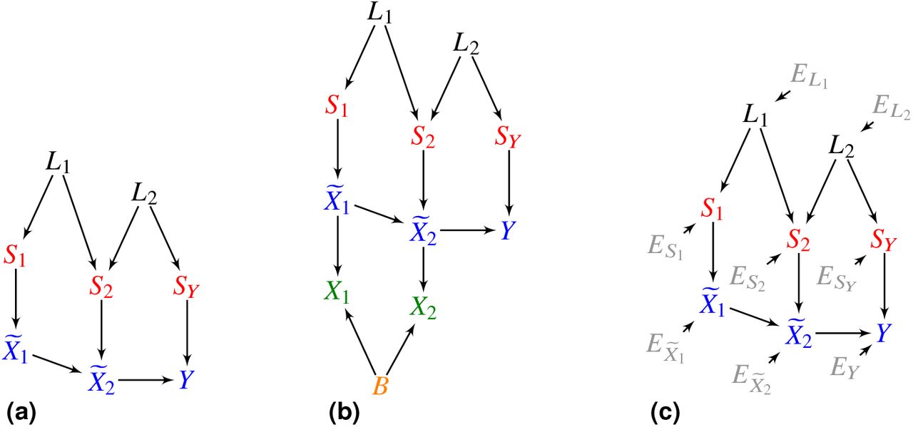
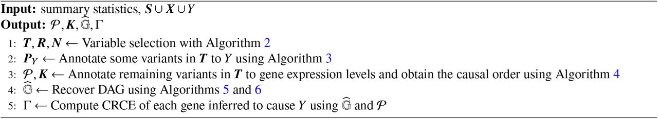
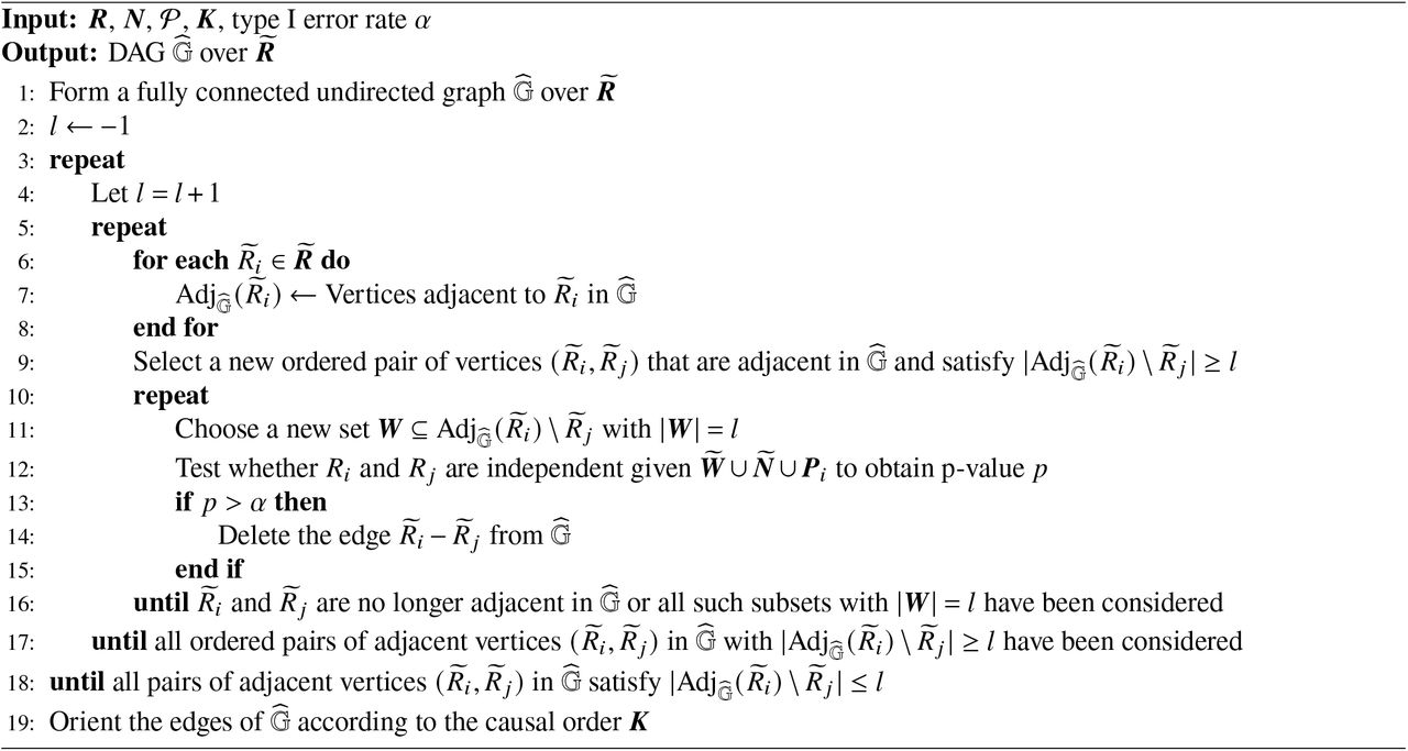References

1.↵
Strobl, E. V. & Gamazon, E. R. Discovering root causal genes with high throughput perturbations. bioRxiv 2024–01 (2024).
2.↵
Boyle, E. A., Li, Y. I. & Pritchard, J. K. An expanded view of complex traits: from polygenic to omnigenic. Cell 169, 1177–1186 (2017).
OpenUrl CrossRef PubMed
3.↵
Martínez-Jiménez, F. et al. A compendium of mutational cancer driver genes. Nat. Rev. Cancer 20, 555–572 (2020).
OpenUrl CrossRef PubMed
4.↵
Strobl, E. V., Lasko, T. A. & Gamazon, E. R. Mitigating pathogenesis for target discovery and disease subtyping. Comput. Biol. Medicine 108122 (2024).
5.↵
Dixit, A. et al. Perturb-seq: dissecting molecular circuits with scalable single-cell rna profiling of pooled genetic screens. Cell 167, 1853–1866 (2016).
OpenUrl CrossRef PubMed
6.↵
Replogle, J. M. et al. Mapping information-rich genotype-phenotype landscapes with genome-scale perturb-seq. Cell 185, 2559–2575 (2022).
OpenUrl
7.↵
Huang, C. et al. Personal transcriptome variation is poorly explained by current genomic deep learning models. Nat. Genet. 55, 2056–2059 (2023).
OpenUrl
8.↵
Sasse, A. et al. Benchmarking of deep neural networks for predicting personal gene expression from dna sequence highlights shortcomings. Nat. Genet. 55, 2060–2064 (2023).
OpenUrl
9.↵
Lousdal, M. L. An introduction to instrumental variable assumptions, validation and estimation. Emerg. Themes Epidemiol. 15, 1 (2018).
OpenUrl CrossRef PubMed
10.↵
Zhao, S. et al. Adjusting for genetic confounders in transcriptome-wide association studies improves discovery of risk genes of complex traits. Nat. Genet. 56, 336–347 (2024).
OpenUrl
11.↵
Rockman, M. V. & Kruglyak, L. Genetics of global gene expression. Nat. Rev. Genet. 7, 862–872 (2006).
OpenUrl CrossRef PubMed Web of Science
12.↵
Giambartolomei, C. et al. Bayesian test for colocalisation between pairs of genetic association studies using summary statistics. PLoS Genet. 10, e1004383 (2014).
OpenUrl CrossRef PubMed
13.↵
Wang, G., Sarkar, A., Carbonetto, P. & Stephens, M. A simple new approach to variable selection in regression, with application to genetic fine mapping. J. Royal Stat. Soc. Ser. B: Stat. Methodol. 82, 1273–1300 (2020).
OpenUrl
14.↵
Chen, C., Ren, M., Zhang, M. & Zhang, D. A two-stage penalized least squares method for constructing large systems of structural equations. J. Mach. Learn. Res. 19, 1–34 (2018).
OpenUrl CrossRef
15.↵
Jiang, Z. et al. Signet: transcriptome-wide causal inference for gene regulatory networks. Sci. Reports 13, 19371 (2023).
OpenUrl
16.↵
Strobl, E. V. & Lasko, T. A. Identifying patient-specific root causes of disease. In Proceedings of the 13th ACM International Conference on Bioinformatics, Computational Biology and Health Informatics, 1–10 (2022).
17.↵
Strobl, E. V. & Lasko, T. A. Identifying patient-specific root causes with the heteroscedastic noise model. J. Comput. Sci. 72, 102099 (2023).
OpenUrl
18.↵
Spirtes, P., Glymour, C. & Scheines, R. Causation, Prediction, and Search (MIT press, 2000), 2nd edn.
19.↵
Wen, Y. et al. Applying causal discovery to single-cell analyses using causalcell. Elife 12, e81464 (2023).
OpenUrl
20.↵
Sakaue, S. et al. A cross-population atlas of genetic associations for 220 human phenotypes. Nat. Genet. 53, 1415–1424 (2021).
OpenUrl CrossRef PubMed
21.↵
Consortium, G. The gtex consortium atlas of genetic regulatory effects across human tissues. Science 369, 1318–1330 (2020).
OpenUrl Abstract/FREE Full Text
22.↵
Barnes, P. J. Inflammatory mechanisms in patients with chronic obstructive pulmonary disease. J. Allergy Clin. Immunol. 138, 16–27 (2016).
OpenUrl CrossRef PubMed
23.↵
Zhou, D. et al. A unified framework for joint-tissue transcriptome-wide association and mendelian randomization analysis. Nat. Genet. 52, 1239–1246 (2020).
OpenUrl CrossRef PubMed
24.↵
Caramori, G. et al. Copd immunopathology. In Seminars in Immunopathology, vol. 38, 497–515 (Springer, 2016).
OpenUrl
25.↵
Kanehisa, M., Furumichi, M., Tanabe, M., Sato, Y. & Morishima, K. Kegg: new perspectives on genomes, pathways, diseases and drugs. Nucleic Acids Res. 45, D353–D361 (2017).
OpenUrl CrossRef PubMed
26.↵
Breiman, L. Classification and regression trees (Routledge, 2017).
27.↵
Verbanck, M., Chen, C.-Y., Neale, B. & Do, R. Detection of widespread horizontal pleiotropy in causal relationships inferred from mendelian randomization between complex traits and diseases. Nat. Genet. 50, 693–698 (2018).
OpenUrl CrossRef PubMed
28.↵
Võsa, U. et al. Large-scale cis-and trans-eqtl analyses identify thousands of genetic loci and polygenic scores that regulate blood gene expression. Nat. Genet. 53, 1300–1310 (2021).
OpenUrl CrossRef
29.↵
Nurwidya, F., Damayanti, T. & Yunus, F. The role of innate and adaptive immune cells in the immunopathogenesis of chronic obstructive pulmonary disease. Tuberc. Respir. Dis. 79, 5 (2016).
OpenUrl
30.↵
West, E. E., Kolev, M. & Kemper, C. Complement and the regulation of t cell responses. Annu. Rev. Immunol. 36, 309–338 (2018).
OpenUrl CrossRef
31.↵
McInnes, L., Healy, J. & Melville, J. Umap: Uniform manifold approximation and projection for dimension reduction. arXiv preprint arXiv:1802.03426 (2018).
32.↵
Ward Jr, J. H. Hierarchical grouping to optimize an objective function. J. Am. Stat. Assoc. 236–244 (1963).
33.↵
Elsworth, B. et al. The mrc ieu opengwas data infrastructure. BioRxiv 2020–08 (2020).
34.↵
Jensen, R. V., Hjortbak, M. V. & Bøtker, H. E. Ischemic heart disease: an update. In Seminars in Nuclear Medicine, vol. 50, 195–207 (Elsevier, 2020).
OpenUrl
35.↵
Bycroft, C. et al. The uk biobank resource with deep phenotyping and genomic data. Nature 562, 203–209 (2018).
OpenUrl CrossRef PubMed
36.↵
Batty, M., Bennett, M. R. & Yu, E. The role of oxidative stress in atherosclerosis. Cells 11, 3843 (2022).
OpenUrl
37.↵
Gan, X. et al. Tag-mediated isolation of yeast mitochondrial ribosome and mass spectrometric identification of its new components. Eur. J. Biochem. 269, 5203–5214 (2002).
OpenUrl CrossRef PubMed Web of Science
38.↵
Chen, W. et al. Tumor protein translationally controlled 1 is a p53 target gene that promotes cell survival. Cell Cycle 12, 2321–2328 (2013).
OpenUrl CrossRef
39.↵
Mostafavi, H., Spence, J. P., Naqvi, S. & Pritchard, J. K. Systematic differences in discovery of genetic effects on gene expression and complex traits. Nat. Genet. 55, 1866–1875 (2023).
OpenUrl
40.↵
Strobl, E. V. Causal discovery with a mixture of dags. Mach. Learn. 1–25 (2022).
41.↵
Yang, W. et al. Promoter-sharing by different genes in human genome–cpne1 and rbm12 gene pair as an example. BMC Genomics 9, 1–16 (2008).
OpenUrl CrossRef PubMed Web of Science
42.↵
Lauritzen, S. L., Dawid, A. P., Larsen, B. N. & Leimer, H.-G. Independence properties of directed markov fields. Networks 20, 491–505 (1990).
OpenUrl
43.↵
Choudhary, S. & Satija, R. Comparison and evaluation of statistical error models for scrna-seq. Genome Biol. 23, 27 (2022).
OpenUrl CrossRef PubMed
44.↵
Sarkar, A. & Stephens, M. Separating measurement and expression models clarifies confusion in single-cell rna sequencing analysis. Nat. Genet. 53, 770–777 (2021).
OpenUrl CrossRef PubMed
45.↵
Bowley, A. The standard deviation of the correlation coefficient. J. Am. Stat. Assoc. 23, 31–34 (1928).
OpenUrl CrossRef
46.↵
Stone, M. Cross-validatory choice and assessment of statistical predictions. J. Royal Stat. Soc. Ser. B (Methodological) 36, 111–133 (1974).
OpenUrl
47.↵
Storey, J. D. The positive false discovery rate: a bayesian interpretation and the q-value. The Annals Stat. 31, 2013–2035 (2003).
OpenUrl
48.↵
Colombo, D., Maathuis, M. H. et al. Order-independent constraint-based causal structure learning. J. Mach. Learn. Res. 15, 3741–3782 (2014).
OpenUrl
49.↵
Cristianini, N. & Shawe-Taylor, J. An introduction to support vector machines and other kernel-based learning methods (Cambridge University Press, 2000).
50.↵
Strobl, E. V., Zhang, K. & Visweswaran, S. Approximate kernel-based conditional independence tests for fast non-parametric causal discovery. J. Causal Inference 7, 20180017 (2019).
OpenUrl
51.↵
Shimizu, S., Hoyer, P. O., Hyvärinen, A., Kerminen, A. & Jordan, M. A linear non-gaussian acyclic model for causal discovery. J. Mach. Learn. Res. 7 (2006).
52.↵
Hoyer, P., Janzing, D., Mooij, J. M., Peters, J. & Schölkopf, B. Nonlinear causal discovery with additive noise models. Adv. Neural Inf. Process. Syst. 21 (2008).
53.↵
Danecek, P. et al. Twelve years of samtools and bcftools. Gigascience 10, giab008 (2021).
OpenUrl CrossRef PubMed
54.↵
Westra, H.-J. et al. Systematic identification of trans eqtls as putative drivers of known disease associations. Nat. Genet. 45, 1238–1243 (2013).
OpenUrl CrossRef PubMed
55.↵
Matthews, B. W. Comparison of the predicted and observed secondary structure of t4 phage lysozyme. Biochimica et Biophys. Acta (BBA)-Protein Struct. 405, 442–451 (1975).
OpenUrl
56.↵
Acid, S. & de Campos, L. M. Searching for bayesian network structures in the space of restricted acyclic partially directed graphs. J. Artif. Intell. Res. 18, 445–490 (2003).
OpenUrl

View the discussion thread.

Posted August 12, 2024.

Download PDF

Data/Code

Citation Tools

Subject Area

Genetic and Genomic Medicine

Subject Areas

All Articles

Addiction Medicine (349)
Allergy and Immunology (668)
Allergy and Immunology (668)
Anesthesia (181)
Cardiovascular Medicine (2648)
Dentistry and Oral Medicine (316)
Dermatology (223)
Emergency Medicine (399)
Endocrinology (including Diabetes Mellitus and Metabolic Disease) (942)
Epidemiology (12228)
Forensic Medicine (10)
Gastroenterology (759)
Genetic and Genomic Medicine (4103)
Geriatric Medicine (387)
Health Economics (680)
Health Informatics (2657)
Health Policy (1005)
Health Systems and Quality Improvement (985)
Hematology (363)
HIV/AIDS (851)
Infectious Diseases (except HIV/AIDS) (13695)
Intensive Care and Critical Care Medicine (797)
Medical Education (399)
Medical Ethics (109)
Nephrology (436)
Neurology (3882)
Nursing (209)
Nutrition (577)
Obstetrics and Gynecology (739)
Occupational and Environmental Health (695)
Oncology (2030)
Ophthalmology (585)
Orthopedics (240)
Otolaryngology (306)
Pain Medicine (250)
Palliative Medicine (75)
Pathology (473)
Pediatrics (1115)
Pharmacology and Therapeutics (466)
Primary Care Research (452)
Psychiatry and Clinical Psychology (3432)
Public and Global Health (6527)
Radiology and Imaging (1403)
Rehabilitation Medicine and Physical Therapy (814)
Respiratory Medicine (871)
Rheumatology (409)
Sexual and Reproductive Health (410)
Sports Medicine (342)
Surgery (448)
Toxicology (53)
Transplantation (185)
Urology (165)

[1] 1.↵
Strobl, E. V. & Gamazon, E. R. Discovering root causal genes with high throughput perturbations. bioRxiv 2024–01 (2024).

[2] 2.↵
Boyle, E. A., Li, Y. I. & Pritchard, J. K. An expanded view of complex traits: from polygenic to omnigenic. Cell 169, 1177–1186 (2017).
OpenUrl CrossRef PubMed

[3] 3.↵
Martínez-Jiménez, F. et al. A compendium of mutational cancer driver genes. Nat. Rev. Cancer 20, 555–572 (2020).
OpenUrl CrossRef PubMed

[4] 4.↵
Strobl, E. V., Lasko, T. A. & Gamazon, E. R. Mitigating pathogenesis for target discovery and disease subtyping. Comput. Biol. Medicine 108122 (2024).

[5] 5.↵
Dixit, A. et al. Perturb-seq: dissecting molecular circuits with scalable single-cell rna profiling of pooled genetic screens. Cell 167, 1853–1866 (2016).
OpenUrl CrossRef PubMed

[6] 6.↵
Replogle, J. M. et al. Mapping information-rich genotype-phenotype landscapes with genome-scale perturb-seq. Cell 185, 2559–2575 (2022).
OpenUrl

[7] 7.↵
Huang, C. et al. Personal transcriptome variation is poorly explained by current genomic deep learning models. Nat. Genet. 55, 2056–2059 (2023).
OpenUrl

[8] 8.↵
Sasse, A. et al. Benchmarking of deep neural networks for predicting personal gene expression from dna sequence highlights shortcomings. Nat. Genet. 55, 2060–2064 (2023).
OpenUrl

[9] 9.↵
Lousdal, M. L. An introduction to instrumental variable assumptions, validation and estimation. Emerg. Themes Epidemiol. 15, 1 (2018).
OpenUrl CrossRef PubMed

[10] 10.↵
Zhao, S. et al. Adjusting for genetic confounders in transcriptome-wide association studies improves discovery of risk genes of complex traits. Nat. Genet. 56, 336–347 (2024).
OpenUrl

[11] 11.↵
Rockman, M. V. & Kruglyak, L. Genetics of global gene expression. Nat. Rev. Genet. 7, 862–872 (2006).
OpenUrl CrossRef PubMed Web of Science

[12] 12.↵
Giambartolomei, C. et al. Bayesian test for colocalisation between pairs of genetic association studies using summary statistics. PLoS Genet. 10, e1004383 (2014).
OpenUrl CrossRef PubMed

[13] 13.↵
Wang, G., Sarkar, A., Carbonetto, P. & Stephens, M. A simple new approach to variable selection in regression, with application to genetic fine mapping. J. Royal Stat. Soc. Ser. B: Stat. Methodol. 82, 1273–1300 (2020).
OpenUrl

[14] 14.↵
Chen, C., Ren, M., Zhang, M. & Zhang, D. A two-stage penalized least squares method for constructing large systems of structural equations. J. Mach. Learn. Res. 19, 1–34 (2018).
OpenUrl CrossRef

[15] 15.↵
Jiang, Z. et al. Signet: transcriptome-wide causal inference for gene regulatory networks. Sci. Reports 13, 19371 (2023).
OpenUrl

[16] 16.↵
Strobl, E. V. & Lasko, T. A. Identifying patient-specific root causes of disease. In Proceedings of the 13th ACM International Conference on Bioinformatics, Computational Biology and Health Informatics, 1–10 (2022).

[17] 17.↵
Strobl, E. V. & Lasko, T. A. Identifying patient-specific root causes with the heteroscedastic noise model. J. Comput. Sci. 72, 102099 (2023).
OpenUrl

[18] 18.↵
Spirtes, P., Glymour, C. & Scheines, R. Causation, Prediction, and Search (MIT press, 2000), 2nd edn.

[19] 19.↵
Wen, Y. et al. Applying causal discovery to single-cell analyses using causalcell. Elife 12, e81464 (2023).
OpenUrl

[20] 20.↵
Sakaue, S. et al. A cross-population atlas of genetic associations for 220 human phenotypes. Nat. Genet. 53, 1415–1424 (2021).
OpenUrl CrossRef PubMed

[21] 21.↵
Consortium, G. The gtex consortium atlas of genetic regulatory effects across human tissues. Science 369, 1318–1330 (2020).
OpenUrl Abstract/FREE Full Text

[22] 22.↵
Barnes, P. J. Inflammatory mechanisms in patients with chronic obstructive pulmonary disease. J. Allergy Clin. Immunol. 138, 16–27 (2016).
OpenUrl CrossRef PubMed

[23] 23.↵
Zhou, D. et al. A unified framework for joint-tissue transcriptome-wide association and mendelian randomization analysis. Nat. Genet. 52, 1239–1246 (2020).
OpenUrl CrossRef PubMed

[24] 24.↵
Caramori, G. et al. Copd immunopathology. In Seminars in Immunopathology, vol. 38, 497–515 (Springer, 2016).
OpenUrl

[25] 25.↵
Kanehisa, M., Furumichi, M., Tanabe, M., Sato, Y. & Morishima, K. Kegg: new perspectives on genomes, pathways, diseases and drugs. Nucleic Acids Res. 45, D353–D361 (2017).
OpenUrl CrossRef PubMed

[26] 26.↵
Breiman, L. Classification and regression trees (Routledge, 2017).

[27] 27.↵
Verbanck, M., Chen, C.-Y., Neale, B. & Do, R. Detection of widespread horizontal pleiotropy in causal relationships inferred from mendelian randomization between complex traits and diseases. Nat. Genet. 50, 693–698 (2018).
OpenUrl CrossRef PubMed

[28] 28.↵
Võsa, U. et al. Large-scale cis-and trans-eqtl analyses identify thousands of genetic loci and polygenic scores that regulate blood gene expression. Nat. Genet. 53, 1300–1310 (2021).
OpenUrl CrossRef

[29] 29.↵
Nurwidya, F., Damayanti, T. & Yunus, F. The role of innate and adaptive immune cells in the immunopathogenesis of chronic obstructive pulmonary disease. Tuberc. Respir. Dis. 79, 5 (2016).
OpenUrl

[30] 30.↵
West, E. E., Kolev, M. & Kemper, C. Complement and the regulation of t cell responses. Annu. Rev. Immunol. 36, 309–338 (2018).
OpenUrl CrossRef

[31] 31.↵
McInnes, L., Healy, J. & Melville, J. Umap: Uniform manifold approximation and projection for dimension reduction. arXiv preprint arXiv:1802.03426 (2018).

[32] 32.↵
Ward Jr, J. H. Hierarchical grouping to optimize an objective function. J. Am. Stat. Assoc. 236–244 (1963).

[33] 33.↵
Elsworth, B. et al. The mrc ieu opengwas data infrastructure. BioRxiv 2020–08 (2020).

[34] 34.↵
Jensen, R. V., Hjortbak, M. V. & Bøtker, H. E. Ischemic heart disease: an update. In Seminars in Nuclear Medicine, vol. 50, 195–207 (Elsevier, 2020).
OpenUrl

[35] 35.↵
Bycroft, C. et al. The uk biobank resource with deep phenotyping and genomic data. Nature 562, 203–209 (2018).
OpenUrl CrossRef PubMed

[36] 36.↵
Batty, M., Bennett, M. R. & Yu, E. The role of oxidative stress in atherosclerosis. Cells 11, 3843 (2022).
OpenUrl

[37] 37.↵
Gan, X. et al. Tag-mediated isolation of yeast mitochondrial ribosome and mass spectrometric identification of its new components. Eur. J. Biochem. 269, 5203–5214 (2002).
OpenUrl CrossRef PubMed Web of Science

[38] 38.↵
Chen, W. et al. Tumor protein translationally controlled 1 is a p53 target gene that promotes cell survival. Cell Cycle 12, 2321–2328 (2013).
OpenUrl CrossRef

[39] 39.↵
Mostafavi, H., Spence, J. P., Naqvi, S. & Pritchard, J. K. Systematic differences in discovery of genetic effects on gene expression and complex traits. Nat. Genet. 55, 1866–1875 (2023).
OpenUrl

[40] 40.↵
Strobl, E. V. Causal discovery with a mixture of dags. Mach. Learn. 1–25 (2022).

[41] 41.↵
Yang, W. et al. Promoter-sharing by different genes in human genome–cpne1 and rbm12 gene pair as an example. BMC Genomics 9, 1–16 (2008).
OpenUrl CrossRef PubMed Web of Science

[42] 42.↵
Lauritzen, S. L., Dawid, A. P., Larsen, B. N. & Leimer, H.-G. Independence properties of directed markov fields. Networks 20, 491–505 (1990).
OpenUrl

[43] 43.↵
Choudhary, S. & Satija, R. Comparison and evaluation of statistical error models for scrna-seq. Genome Biol. 23, 27 (2022).
OpenUrl CrossRef PubMed

[44] 44.↵
Sarkar, A. & Stephens, M. Separating measurement and expression models clarifies confusion in single-cell rna sequencing analysis. Nat. Genet. 53, 770–777 (2021).
OpenUrl CrossRef PubMed

[45] 45.↵
Bowley, A. The standard deviation of the correlation coefficient. J. Am. Stat. Assoc. 23, 31–34 (1928).
OpenUrl CrossRef

[46] 46.↵
Stone, M. Cross-validatory choice and assessment of statistical predictions. J. Royal Stat. Soc. Ser. B (Methodological) 36, 111–133 (1974).
OpenUrl

[47] 47.↵
Storey, J. D. The positive false discovery rate: a bayesian interpretation and the q-value. The Annals Stat. 31, 2013–2035 (2003).
OpenUrl

[48] 48.↵
Colombo, D., Maathuis, M. H. et al. Order-independent constraint-based causal structure learning. J. Mach. Learn. Res. 15, 3741–3782 (2014).
OpenUrl

[49] 49.↵
Cristianini, N. & Shawe-Taylor, J. An introduction to support vector machines and other kernel-based learning methods (Cambridge University Press, 2000).

[50] 50.↵
Strobl, E. V., Zhang, K. & Visweswaran, S. Approximate kernel-based conditional independence tests for fast non-parametric causal discovery. J. Causal Inference 7, 20180017 (2019).
OpenUrl

[51] 51.↵
Shimizu, S., Hoyer, P. O., Hyvärinen, A., Kerminen, A. & Jordan, M. A linear non-gaussian acyclic model for causal discovery. J. Mach. Learn. Res. 7 (2006).

[52] 52.↵
Hoyer, P., Janzing, D., Mooij, J. M., Peters, J. & Schölkopf, B. Nonlinear causal discovery with additive noise models. Adv. Neural Inf. Process. Syst. 21 (2008).

[53] 53.↵
Danecek, P. et al. Twelve years of samtools and bcftools. Gigascience 10, giab008 (2021).
OpenUrl CrossRef PubMed

[54] 54.↵
Westra, H.-J. et al. Systematic identification of trans eqtls as putative drivers of known disease associations. Nat. Genet. 45, 1238–1243 (2013).
OpenUrl CrossRef PubMed

[55] 55.↵
Matthews, B. W. Comparison of the predicted and observed secondary structure of t4 phage lysozyme. Biochimica et Biophys. Acta (BBA)-Protein Struct. 405, 442–451 (1975).
OpenUrl

[56] 56.↵
Acid, S. & de Campos, L. M. Searching for bayesian network structures in the space of restricted acyclic partially directed graphs. J. Artif. Intell. Res. 18, 445–490 (2003).
OpenUrl

Transcriptome-Wide Root Causal Inference

ABSTRACT

1 Introduction

2 Results

2.1 Overview of TWRCI

2.1.1 Setup

2.1.2 Variable Selection

2.1.3 Annotation by Competitive Regression

2.1.4 Causal Discovery and CRCE Estimation

2.2 TWRCI accurately annotates, reconstructs and estimates in silico

2.3 Adaptive immunity in COPD

2.3.1 Accuracy

2.3.2 Horizontal pleiotropy and trans-variants

2.3.3 Root Causal Mechanism

2.4 Oxidative stress in ischemic heart disease

2.4.1 Accuracy

2.4.2 Horizontal pleiotropy and trans-variants

2.4.3 Root Causal Mechanism

3 Discussion

Data Availability

4 Methods

4.1 Background on Causal Discovery

4.2 Causal Modeling of Variants, Gene Expression and the Phenotype

4.3 Conditional Root Causal Effects

4.4 Algorithm

4.4.1 Strategy Overview

Transcriptome-Wide Root Causal Inference (TWRCI)

4.4.2 Variable Selection

Variable Selection

4.4.3 Annotation for Horizontal Pleiotropy

Competitive Regression (CR)

4.4.4 Annotation and Causal Order

Annotation and Causal Order (ACO)

4.4.5 Causal Graph Discovery

Graph Discovery

CRCE Graph Discovery

4.4.6 Conditional Root Causal Effect Estimation

4.4.7 Time Complexity

4.5 Comparators

Annotation

Causal Graph Reconstruction

4.6 Semi-Synthetic Data

4.7 Real Data

4.7.1 Data Availability

4.7.2 Quality Control

4.7.3 Comparison to trans-eQTLs

4.8 Metrics

4.9 Code Availability

5 Supplementary Materials

5.1 Additional Semi-Synthetic Data Results

5.2 Additional COPD Data Results

5.3 Additional IHD Data Results

5.4 Proofs

Acknowledgements

Footnotes

References

Citation Manager Formats

Subject Area